Event Related Tutorial

This tutorial will show you how to run an event-related analysis. Note that the Retinotopy Tutorial is the best place to start for a full introduction to using mrLoadRet. This tutorial starts after the initial steps of running mrInit, the Motion Compensation and Alignment – those steps are described in the retinotopy tutorial. The experiment that is being analyzed here is one in which the subject viewed randomly moving dots. On each trial, the dots moved coherently for a couple of seconds in one of three directions, and then went back to moving incoherently for several seconds. Thus there are three different trial types that will be deconvolved, for each of the three directions of motion, and we will look at the responses in MT.

1. Download the tutorial files
2. Concatenate scans together
3. Set stimfiles
4. Run event-related analysis
5. Viewing the analysis

You can download the tutorial files from:

erTutorial.tar.gz

Note that this is a rather large file. Approximately 300MB.

The files are provided as a tar/zip file. In Mac OS X you should be able to just click to open the files in the Finder. Otherwise, you can go to a terminal and do:

gunzip erTutorial.tar.gz
tar xvf erTutorial.tar

We assume that you have mrTools running on your system.

Start up Matlab and switch to the erTutorial directory you just downloaded, and run mrLoadRet:

cd erTutorial
mrLoadRet

We are going to run a concatenation. The purpose of concatenating scans together is first to make a single long scan out of a few shorter scans so that we can estimate the responses using all the data. Second, this step runs preprocessing steps on the data such as high-pass filtering and converting to percent signal change.

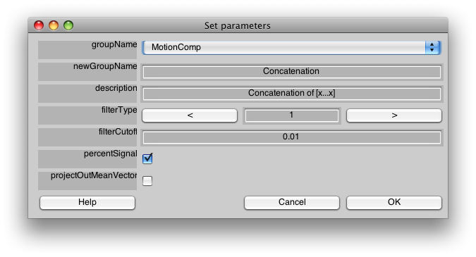
Make sure the Group tab is set to MotionComp and then Select Concatenate Time Series from the Analysis menu. You should see a dialog like the following:

We do not need to change anything on this dialog to have it run. For a description of the meaning of the parameters press help, or see the Event Related manual pages.

Press OK.

You will see another dialog where you should select all the scans for concatenating:

Press OK. This will take a few minutes to run.

We will now tell mrLoadRet which “stimfiles” to use for these scans. Stimfiles contain the information about the timing of events in the experiment that is used for the deconvolution analysis. Note that we set the stimfiles on the Raw TSeries (i.e. the original time series). This can be done before or after the concatenation is done. The concatenation scan has saved what original scans and from what group it came from. So, to find the correct stimfiles, mrLoadRet always checks back to those scans to see what stimfiles they are linked to. This way, you can always change how you have linked the stimfiles at any given time.

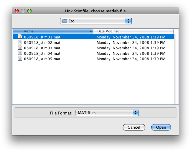
Switch the Group tab to Raw. Go to Scan 1. Now go to the Edit menu and select Edit/Scan/Link Stimfile. You should get a file choosing dialog like this:

Choose to link the first scan with the first stimfile “stimvol01.mat” and click Open.

Now, Set the scan slider to 2, and repeat this process, linking scan 2 with stimvol02.mat.

Link all the rest of the scans accordingly, (i.e. Scan 3 → stimvol03, Scan 4 → stimvol04 and Scan 5 → stimvol05).

While this is a bit tedious, the process can be automated for a real experiment you run, and the mrInit dialog makes it easier to link all the stimfiles at one time when you first start your session.

Now, let's go check to make sure that you have linked the files correctly.

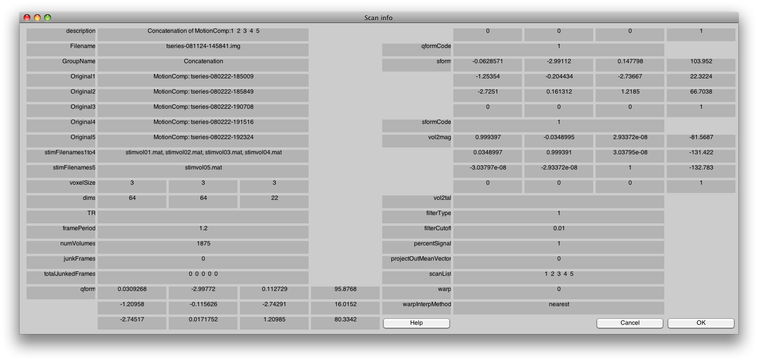
Switch to the Concatenation Group, and then choose the Edit/Scan/Info menu item.

You should see something like the following:

In particular, check that the stimFilenames are listed in sequential order. If they are not, switch back to the Raw group and fix it by re-linking the stimfiles again.

The stimfile format used here is very simple. It is a cell array where each element in the cell array is for a different trial type (in this case different directions of dot motion). Each element of the cell array consists of an array whose elements list the volume number that the stimulus occurred on. There is also a stimNames cell array that gives what the names of the trial types are. You can see what this looks like, by doing (from the matlab command line);

v = newView;
stimfile = viewGet(v,'stimfile',1,1);

and you should see that it looks like:

  >> stimfile{1}

ans = 

      stimvol: {[21 38 60 75 96 104 150 156 181 195 223 256 285 300 305 332 364]  [1x18 double]  [1x17 double]}
    stimNames: {'Direction: 35 deg'  'Direction: 135 deg'  'Direction: 255 deg'}
     filetype: 'stimvol'

For a description on how to create your own stimfiles see the Event Related manual pages.

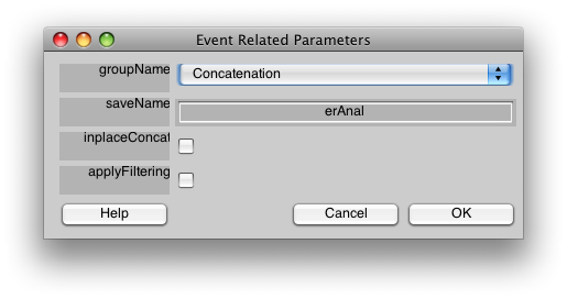
Now, let's run the event-related analysis. Select Event-related analysis from the Analysis menu, and you should see the following dialog:

You should select “applyFiltering”. This checkbox filters the columns of the event-related design matrix in the same way that the data have been filtered (i.e. high-pass filtering). Click OK.

Select the single scan in the next dialog box, and click OK.

You should now see:

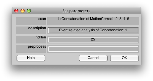
This is the dialog which chooses some information about how to do the event-related analysis. The hdrlen is the length (in # of vols) of the response to calculate in the deconvolution.

Click OK.

Running the analysis will take a few minutes. Note that if you are on a system that does not have very much memory, you can choose to have mrLoadRet break up the computation into smaller chunks. This is set in the Edit/Preferences dialog. The smaller the chunks the longer it will take to calculate, but use less memory.

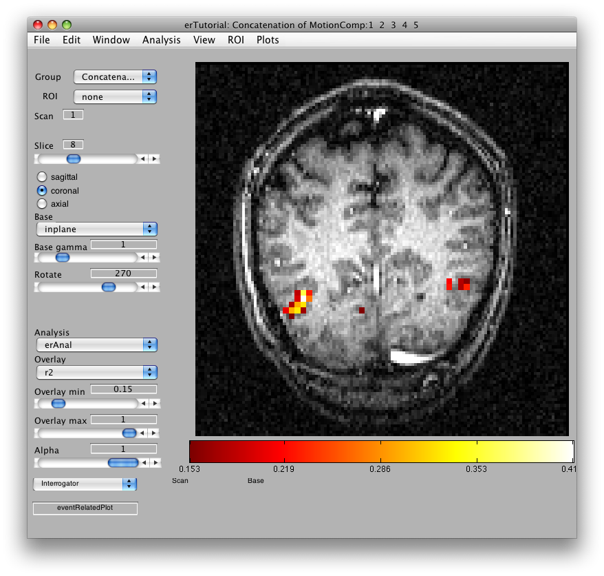
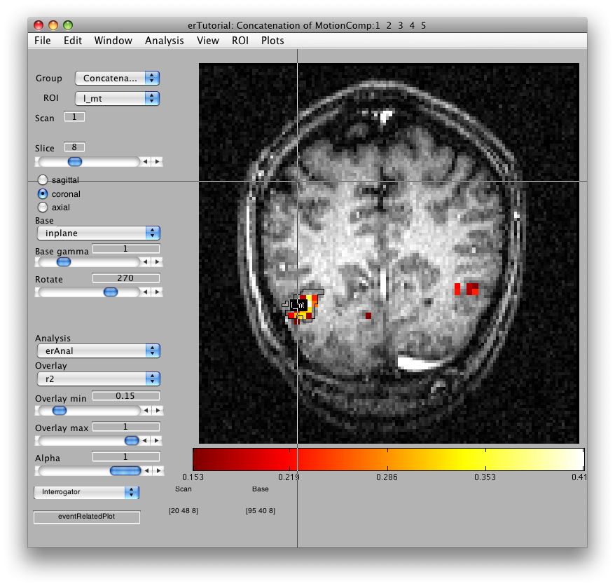
Once the analysis is complete, set the overlay min to 0.2 and the Slice slider to 8, and you should something like the following:

This is an r2 map of the event-related analysis. It tells you what proportion of the variance in each timecourse is accounted for by the average hemodynamic response See Gardner et al., Neuron (2005) 47:607-20, for more information.

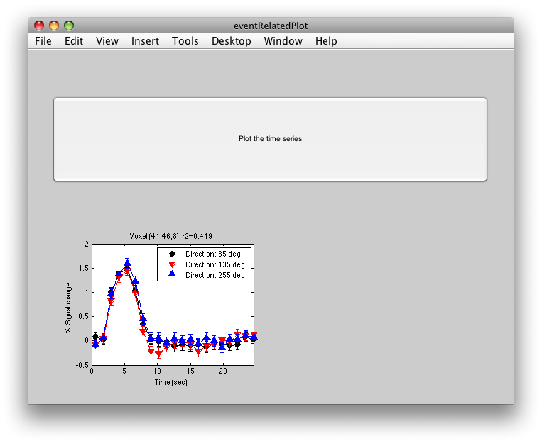
To see what the responses look like at any individual voxel, turn on the interrogator (Plots/Interrogate Overlay) and you should see “eventRelatedPlot” in the text box in the bottom left (see above figure). Go ahead and move the cross-hairs over the voxel with the highest r2 value (white) and click. You should then see:

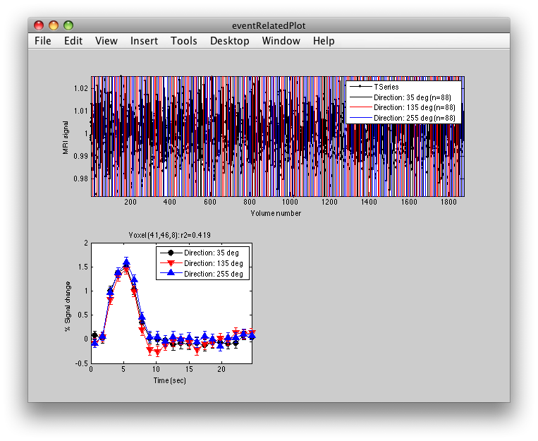
This shows the three deconvolved responses to the three different trial types. If you click on the button to Plot the time series, you will see:

This shows the time series at the top, with a vertical line every time one of the trials occurred. Note that the time course is in percent signal change, and has been set to have a mean of 1. This is what the concatenation code does. The mean is set to 1, so that if you divide by the mean again (to get percent signal change), nothing will change in the time series.

You can also look at average responses across an ROI. To do that, load the l_mt roi, by using File/ROI/Load. You should now see:

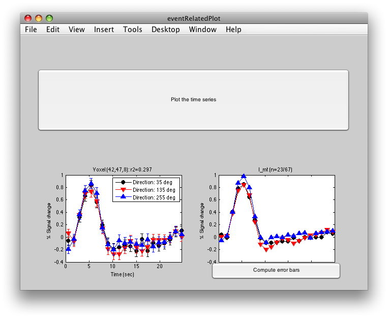
Click inside the l_mt roi and you will get:

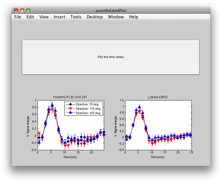
The graph on the left shows the individual voxel you clicked on. The graph on the right shows the deconvolution averaged across all the voxels in the l_mt ROI that meet the r2 cutoff that you set in the Overlay Min. This display simply averages across the already computed deconvolved responses. If you want to get error bars, click the “Compute Error bars” button, and after a little bit, you should see:

What this does, is reloads all the time courses that meet the r2 cutoff set by the overlay min and then averages those time courses together into a single time course. It then recomputes the deconvolution analysis on this average time course. The error bars are now standard errors over the number of repeats of the stimulus. (Technically, they are computed as the residual variance distributed back to each time point in the deconvolved response according to the inverse of the covariance of the design matrix).

-jg.