Table of Contents
Introduction
Encoding models can be a powerful way to analyze data because they can reduce a high-dimensional stimulus space to a lower dimensional representation based on knowledge of how neural system encode stimuli and thus have more power to extract relevant information from cortical measurements. A channel encoding model, first introduced by Brouwer & Heeger, 2009 for the representation of color has been widely used to understand cortical representations of continuous stimulus variables like orientation, direction of motion and space. This tutorial will teach you how to simulate data for oriented stimuli that conform to the assumptions of the model, fit and invert the model.
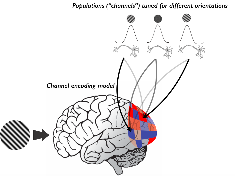
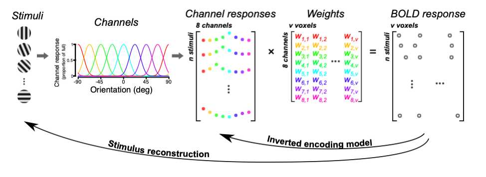
The basic idea is that each measurement unit (typically a voxel) is modeled to be the linear sum of underlying populations of neurons tuned for different orientations. So, for example if you present some orientation and get responses higher (red) or lower (blue) than the mean response, you would assume that higher responses are due to a stronger weighting of neural populations tuned for that orientation, and weaker responses due to stronger weighting of neural populations tuned for other orientations.
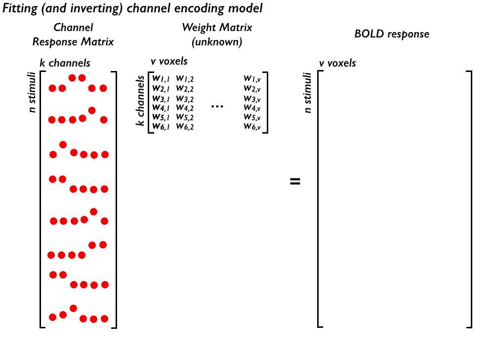
In matrix algebra, what one does is make a channel response matrix which contains the channel responses for each of the stimuli in an experiment (one row per trial). This gets multiplied by an (unknown) weight matrix that best fits the measured BOLD responses (one row for each stimulus). Note that typically you need to get a single amplitude for each voxel per trial. This can be done simply by taking a single time point at the peak of response, averaging over some time window or fitting a hemodynamic response function and computing the magnitude of that. For this tutorial, we will assume that you have a single scalar response for each voxel for each trial already computed. The matrix tableaux looks like this:
In the forward encoding, one solves for the weight matrix typically by doing a least-squares regression. In inverse encoding, one uses this estimated weight matrix to invert the equation and solve for the channel responses.
Learning goals
After finishing this tutorial you will be able to
- simulate data for fitting a channel encoding model
- perform forward encoding by fitting the weight matrix to simulated data
- compute the goodness-of-fit of the model
- invert the encoding model
- use a simplified Bayesian algorithm to determine the stimulus likelihood
- understand that the channel basis functions are only constrained up to a linear transform
Note that this tutorial is self-paced and designed so that you can copy-and-paste code as you go along. The code does not require any libraries or complex functions so, if you are so inclined, you might try writing the code yourself (without looking at the Matlab cheat sheets below). If you are a python (or other language) kind of person, you could easily write the code in another programming language. If you do, send me (Justin) the code and I will add it to the tutorial! All the code appears behind hidden tabs. If you want to grab the whole code set, you can find it here.
Thanks to João Guassi Moreira there is an R Markdown version of the script here which can be previewed in html here!
Simulated data
First let's simulate some data. Later you will see this done on real data, but it's *always* a good idea to run your analyses on simulations where you know the ground truth to test how your model behaves. So, let's start with some basic assumptions about how the model works. The model assumes that each voxel (or EEG electrode or whatever measurement you are making) is a linear sum of individual channels that are tuned for some stimulus feature. We will do this here with orientation as the feature, but this can and has been done with other features (direction of motion, space or really anything in which you can define a tuning function that is reasonable given what you know about the neural representation).
Start, by making a matrix called neuralResponse in which you have 90 neurons (one per row of the matrix) and in each column it's ideal response to one of 180 orientations. Let's assume that the neurons are tuned according to a Von Mises function which is often used as a circular equivalent to a Gaussian. Each neuron will be tuned to a different orientation. Why 90 neurons? Just so that we can keep the matrix dimensions clear. Half the battle with linear algebra is getting your matrix dimensions right after all.
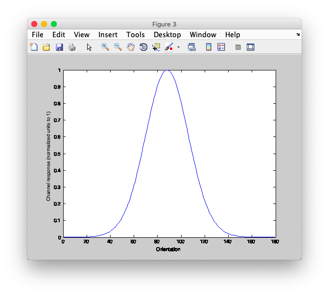
If you got that working then, you should be able to plot a single neuron response function, let's try the 45th neuron - which should be tuned to 90 degees.
Should look like the following.
Ok. Now we want to simulate v voxels (say 250) response as random combinations of the neural tuning functions. The basic idea is that each voxel contains some random sub-populations of neurons tuned for different orientations and the total response is just a linear combination of these. So, let's make a random matrix that are the weights of each of these neurons onto each voxel. This should be a matrix called neuronToVoxelWeights that is nNeurons x nVoxels in size where each column contains ranodom weights for each voxel.
Now, let's simulate an experiment in which we have nStimuli of different orientations. To keep things simple, we will have nStimuli=8 stimuli that are evenly spaced across orientations starting at 0. And we will have nRepeats (say 20) of each stimuli. In a real experiment, we would randomize the order of the stimuli so as to avoid adaptation and other non-stationary effects, but here we can just have them in a sequential order. We can start by making an array stimuli of length nStimuli x nRepeats with the stimulus values.
A few simple things here - let's round all the stimulus values to the nearest integer degree (just for ease of calculation) and add one (because Matlab indexes starting with one and not zero) and make this into a column array
ok, now we can compute the response to each stimulus. So we should make a voxelResponse matrix (dimensions nTrials = nStimuli x nRepeats by nVoxels).
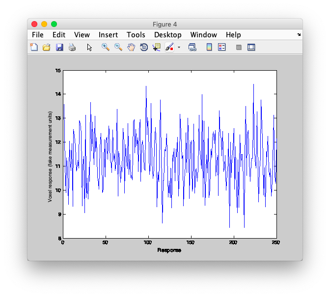
Great. let's see what we got. Plot the response to, say trial 7
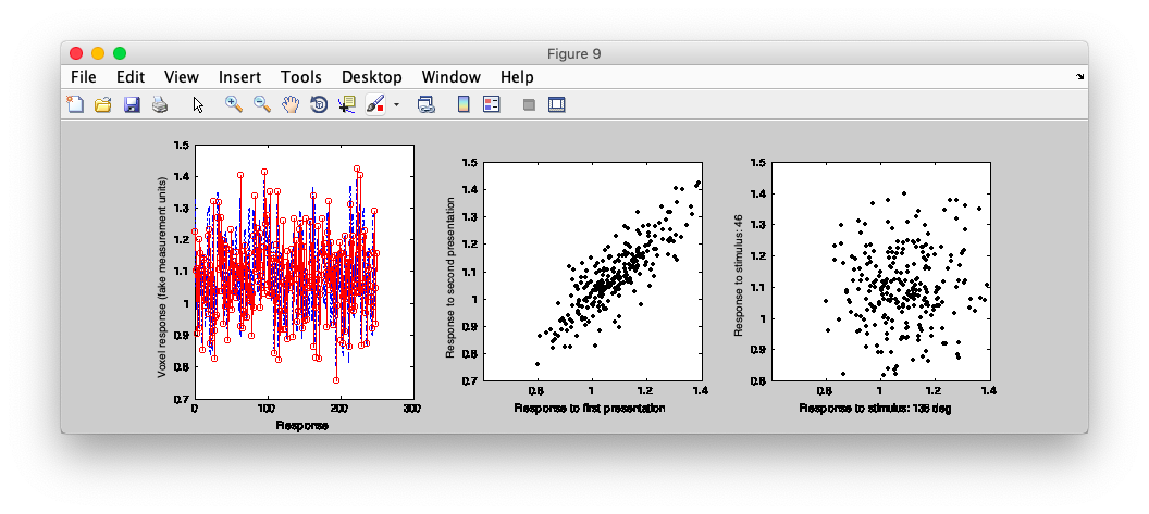
Now, plot another trial that is in response to the same stimulus on top of that. See any problem?
Ok. Let's fix that by adding random gaussian noise to the voxelResponses (BTW - this is a a very simple noise model called IID - independent, identically distributed gaussian noise - in reality, noise is going to have some complex characteristics, for example, there might be more correlation between neighboring voxels than voxels spatially distant - or more correlation between voxels that receive similarly tuning - but for this purpose, let's go with this simple nosie model). Just to keep the scale understandable, let's normalize the voxel responses to have a mean of 1 and then add gaussian noise with a fixed noiseStandardDeviation of, say, 0.05.
Always check your work - now two responses should not be identical, but correlated. And not correlated with responses to very different orientations.
Okey, dokey. We now have a simulated voxelResponse that we can test our model with. Remember, that everything that we did in the simulation is an assumption: Von Mises tuned neurons, random linear weighting, IID noise and SNR (signal-to-noise ratio as in the magnitude of the orientation tuned response compared to the noise). Each of these may or may not be valid for real data and should ideally be tested (or at least thought about deeply!). The beauty of a simulation is that we can change these assumptions and see how they affect the analysis - something that is really, really important to do as you learn about new analysis techniques. If the assumptions are incorrect, the analysis can fall apart in ways that are often unexpected and you may infer incorrect conclusions, so play around with these simulations first to understand what is going on!
Encoding model
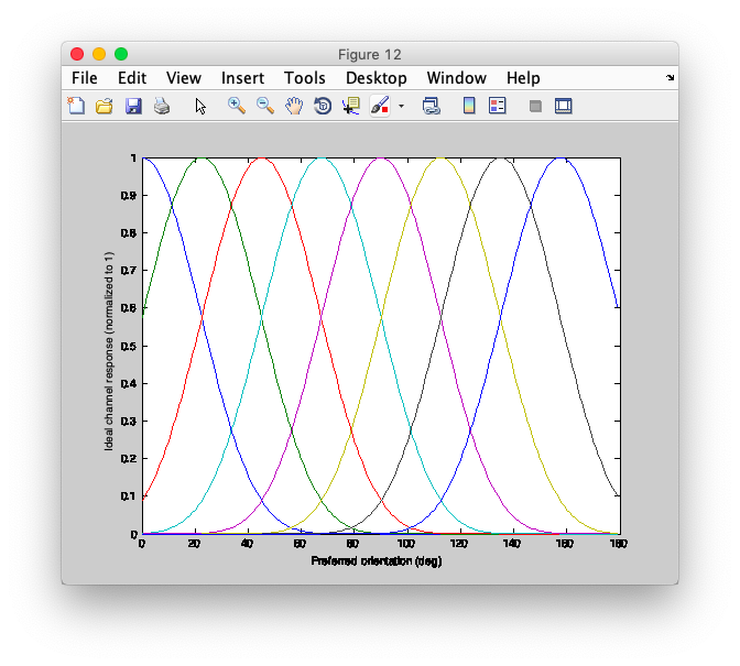
Ok, let's build the encoding model. In this case we are going to assume that there are nChannels = 8, that are tuned as exponentiated and rectified sinusoids to different orientations. Note that this is different from the assumptions above of Von Mises tuned neurons. Will get back to that later! Let's build a matrix called channelBasis which is 180 x nChannels that contains the ideal channel responses (also called channel basis functions) to each of 180 orientations. We will use gaussian functions raised to the exponent 7.
Ok. If that worked, then we should have 8 channels that are tuned for different orientations. Let's plot it to make sure!
Should look like the following:
Great. Now, let's compute responses of these idealized channel basis functions to each one of th nTrials in the array stimuli. We will compute a nTrial x nChannel matrix called channelResponse
Easy, right? Now let's fit this model to the simulated data. Remember that the model that we have is: channelResponses (nTrials x nChannels) x estimatedWeights (nChannels x nVoxels) = voxelResponses (nTrials x nVoxels) You can solve this by doing your favorite least-squares estimation procedure (or if you want to be fancy, you could do some robust regression technique). We'll just do the basic here.
Model fit
Whenever you fit a model, it's always important to compute a measure of model fit - how well does the model actually fit the data. r2, amount of variance accounted for, is a good measure for this sort of data. So, compute that by seeing what the model predicts for the data (that's easy, that's just channelResponse x estimatedWeights and remove that from the data. Then compute 1 minus the residual variance / variance.
You should get a pretty good r2 value (like over 80-90% of variance accounted for). That would be terrific for real data - great working with a simulation, right?
Inverted encoding model
Ok. Now, let's invert the model to see what it predicts for channel responses. But, first we gotta talk about cross-validation. Always, always cross-validate. There, we are done talking about it. Here, let's do a simple version where we split the data into two (split-half cross-validation). Make two matrices from your voxelData where trainVoxelResponse is the first half trials and testVoxelResponse is the second half. Then compute estimatedWeights on the trainVoxelResponse.
Now on the second half of the data, compute the estimatedChannelResponse (look at above equations for channelResponses and use least-squares estimation
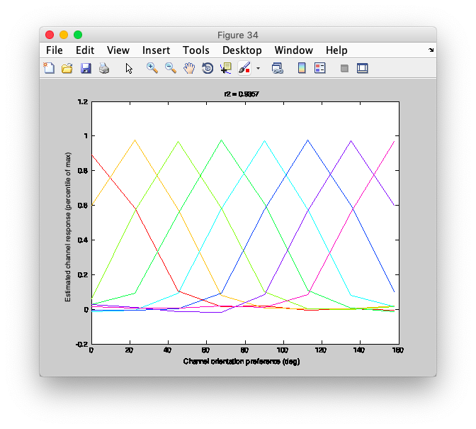
Ok. Let's see what we've got. Plot the mean estimatedChannelResponse for each stimulus type
Should look like the following
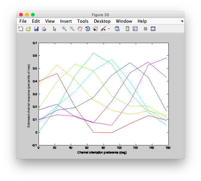
Maybe, a little too pretty. Try the whole simulation again, but this time add more noise (try, say an order of magnitude larger noise standard deviation - 0.5) and see what happens to the estimated channel response profiles. Make sure to keep the original low noise voxelResponses by naming the new voxelResponses something different like voxelResponseNoisy
This should make estimated channel response profiles that are more realistic
Break here
For UCSB Brain Camp, if you get to this point, take a break and let us know. We'll explain the stimulus likelihood part with a few slides.
Stimulus likelihood
In the above, an important distinction is that we are inverting to estimate the model responses and not the stimulus itself. There are some cases where this may be exactly what we want, for example, when we model responses as linear combinations of target and mask or when we want to know about off-target gain. But, often what we really want to know is what the population (given our model) tells us about the stimulus. To be clear, there is distinction between reconstructing the model and reconstructing the stimulus.
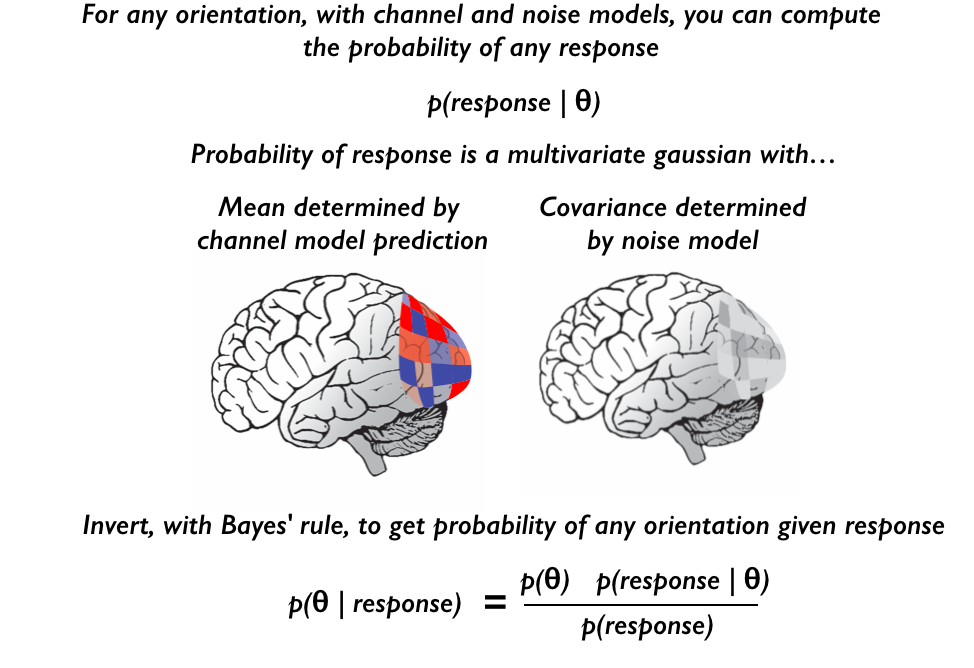
We can do this using a Bayesian analysis that creates a stimulus likelihood function - that is a function that tells you the probability of any stimulus given a particular response . For this, we need to model not just the mean response which the encoding model above does, but also the variance around that mean response.
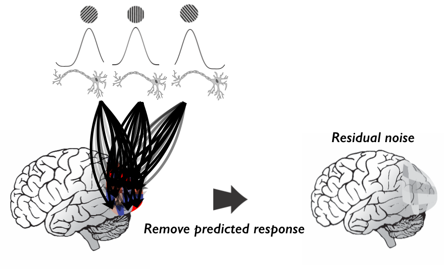
The basic idea is to look at the residuals after you have fit the encoding model. That is, one removes the prediction of the channel encoding model by subtraction and looks at the residuals:
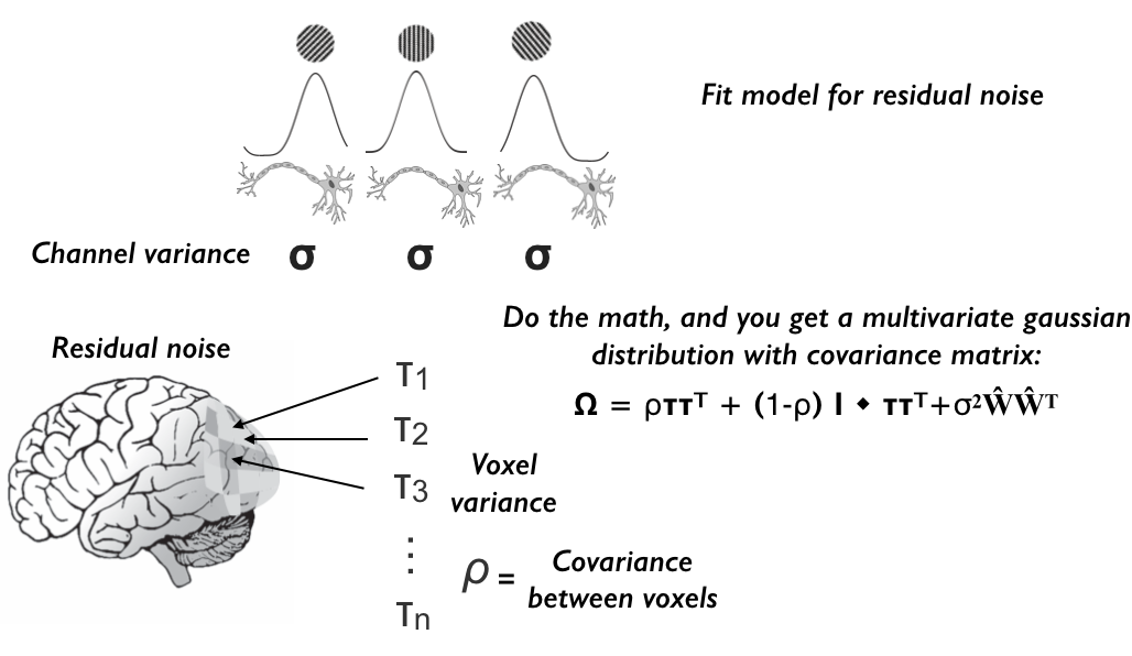
In particular, one wants to fit a multi-variate gaussian noise model to these residuals. In Van Bergen & Jehee, 2015 they use a noise model which has individual variances on each voxel, covariance across voxels and variance on each one of the channels:
Once you know this you can figure out the probability of any stimulus given the measured response, by seeing where that response lives in the multivariate gaussian who's mean is the channel encoding model prediction for that orientation and whose covariance is modeled with the above equations:
For the purpose of this tutorial, we will just model the noise as independent, identically distributed gaussian noise on each voxel. Of course, this is probably wrong, as voxels may have different amount of variation and will have covariation with each other - both due to spatially local effects and to common sources of signal. All of this has been modeled elegantly and validated in Van Bergen & Jehee, 2017.
To compute our simple noise model, we just get the residual variance on each voxel after fitting the encoding model. So, look at the residual, voxel-by-voxel and compute the variance.
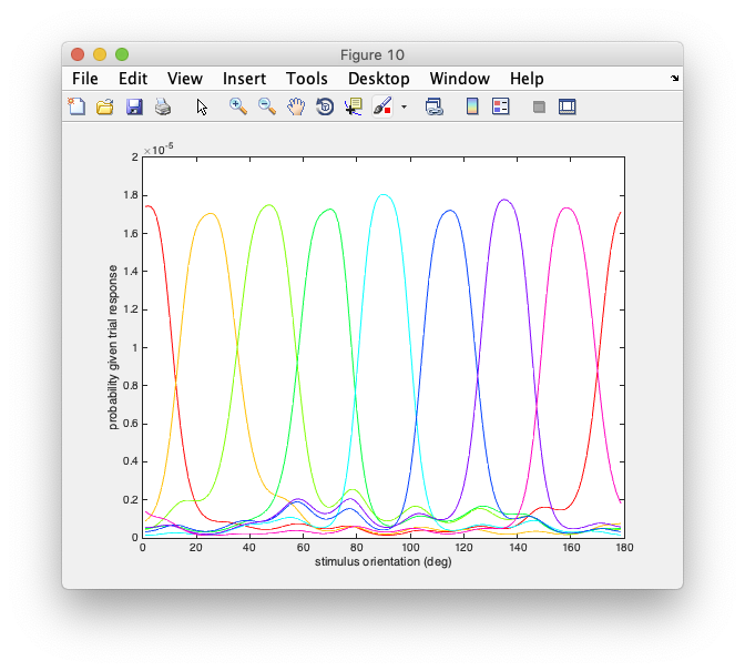
Ok, now we have our full model. The weights give you the mean response expected for any orientation stimulus and the covariance matrix tells us the variation around that mean. So, now if we want to figure out the probability of seeing any test response given any orientation, we simply compute the probability as a multivariate gaussian probability distribution
Should look like something like this:
Inverted Encoding model with different channel basis functions
Now, let's do a little trick. We're going to show that the channel basis functions in the simple inverted encoding model above are only constrained up to a linear transform, which means that you can recreate channel response profiles of arbitrary shapes (as long as they are linearly transformable from the original unimodal exponentiated half-sinusoids we used).
First, we will design a transformation matrix that will convert are original channel basis functions into bimodal ones. Can you figure out an 8×8 transform that will do that?
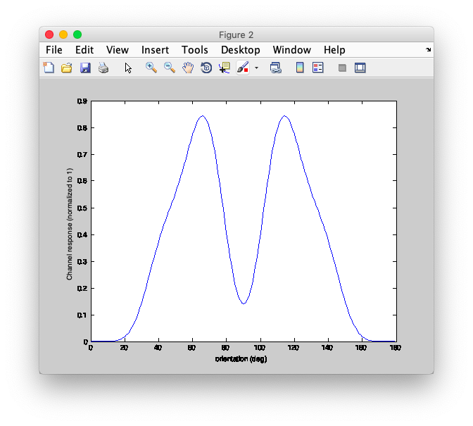
Now, take a look at those channels
Should look like this
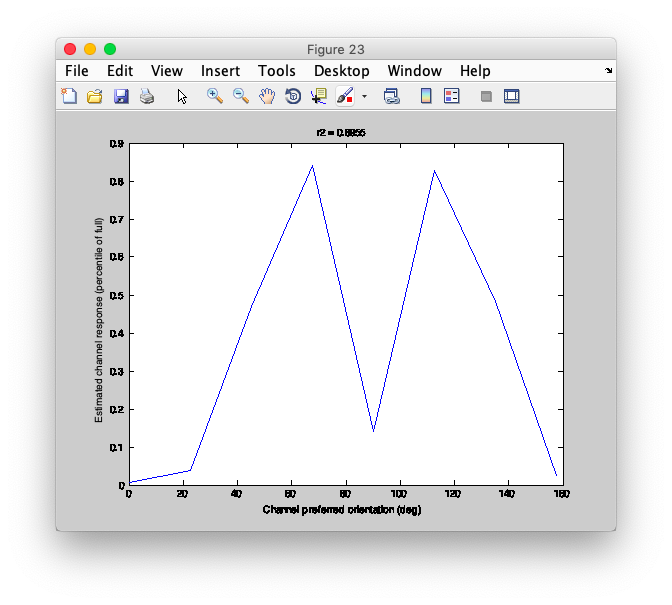
Ok, now fit this model to the data and invert - remember, we are not changing anything about the data, we are just changing the model we are using to analyze the data.
Should look like the following
Remember, there was nothing in our simulated data that was bimodal. The bimodal channel response functions that we get out are simply because we modeled the responses in this way. You get out what you put in. And in this case, since the channel basis functions are linearly related to the original ones we used, they account for exactly the same amount of variance - since they span the same subspace.
Ok. So, we need to be careful about what to interpret when we invert to get the model back. That is, when we do that, we get back the model that we put in. If we use the Bayesian model from above, we can avoid the ambiguity with the channel basis functions. Compute the Bayesian model with this bimodal basis set and you will see that you get back a unimodal likelihood function.
To compute our simple noise model, we just get the residual variance on each voxel after fitting the encoding model. So,
Should look like something like this:
