Retinotopy Tutorial

This tutorial shows you how to run a retinotopy analysis with mrLoadRet. It is a good place to start if you are just learning how to use mrLoadRet.

1. Download the tutorial files
2. The stimuli used in the experiment
3. Make the directory structure for mrLoadRet and move the files into the correct locations
4. Run mrInit to initialize the session
5. Run the Motion Compensation
6. Average wedge and ring scans together
7. Run the correlation analysis
8. Use mrAlign to align the 2D inplane anatomy to the 3D volume anatomy
9. View the results on a flattened representation of occipital cortex
10. Draw the visual area ROIs

You can download the tutorial files from:

retinotopyTutorial.tar.gz

Note that this is a rather big file, approximately 300MB.

The files are provided as a tar/zip file. In Mac OS X you should be able to just click to open the files in the Finder. Otherwise, you can go to a terminal and do:

gunzip retinotopyTutorial.tar.gz
tar xvf retinotopyTutorial.tar

We provide you with a set of 10 functional scans, an inplane anatomy file, a high-resolution T1-weighted volume anatomy used for alignment and a flat map of the right occipital cortex to visualize the results on.

The functional scans include 6 rotating wedge runs (3 CW and 3 CCW rotations) and 4 expanding and contracting ring runs (2 expanding and 2 contracting). Each run is 168 volumes long (a volume was acquired every 1.5 seconds). The first 8 volumes will be thrown out to allow hemodynamic response and longitudinal magnetization to reach steady state. The data has already been motion compensated (since this step takes quite a bit of time to run).

From here, all the directions will be for commands to run under Matlab. It is assumed that you have properly set up mrTools using the directions under Getting Started.

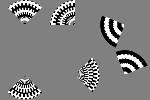
The visual stimuli were run using the mglDoRetinotopy command in the mgl library. A CCW wedge run looks something like the following (though the animating gif probably doesn't play at the right speed – each cycle should take 24 seconds).

The rings stimuli look something like this:

Now that you have the raw image files, you need to make the directory structure for mrLoadRet and copy your files into the correct directories. (Note that this does not have to be done in Matlab, it can be done from the command line or from the Finder or from a shell script that is customized for the file types at your site).

1. Start up Matlab and change directories into the downloaded tutorial data directory

     cd retinotopyTutorial

2. Now make a directory for the anatomy files and move the anatomies into that directory.

     mkdir Anatomy
     movefile inplane.* Anatomy
     movefile volume.* Anatomy
     movefile right_occipital.* Anatomy

3. Now make the directory to hold your raw time series (i.e. the epi scans with your data), and move the scan files into that directory

     mkdir Raw
     mkdir Raw/TSeries
     movefile Scan* ./Raw/TSeries

You should now have two top level directories (Anatomy and Raw) and all the files should have been moved into one of the sub-directories:

>> ls
Anatomy/     Raw/

Now you are ready to run mrInit which will setup your mrLoadRet session:

mrInit

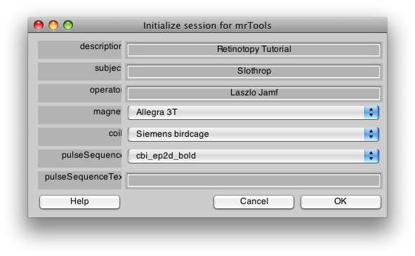
You will first see a dialog like the following. Go ahead and fill in the fields to match what is shown here. This is information about the scan, it is used only for documentation, so you will usually fill in the fields appropriately for the scan you are running. Also, if you are using a different magnet and coil than the one at NYU, you can see the section mrInit on how to customize this dialog to your site. Finally, you may always change this information later, from the mrLoadRet GUI. When you are done, click OK.

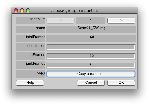
Now you will get a dialog to set the parameters for each scan in the session. For these we are going to give a name to each scan (either CW, CCW, Expanding, or Contracting), and set the number of junkFrames to 8. The junkFrames mean to throw out the first 8 frames of the scan, we do this because we always take an extra half cycle of the stimulus (16 volumes per cycle), to allow both the longitudanal magnetization and hemodynamic response to reach steady-state. Let's start by setting all the scans to have junkFrames of 8. We can do this by putting 8 into the junkFrames field and then pressing “Copy parameters”:

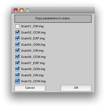
Select all the rest of the scans. This is the quickest way to copy the junkFrames parameter to all of those scans. Press Ok.

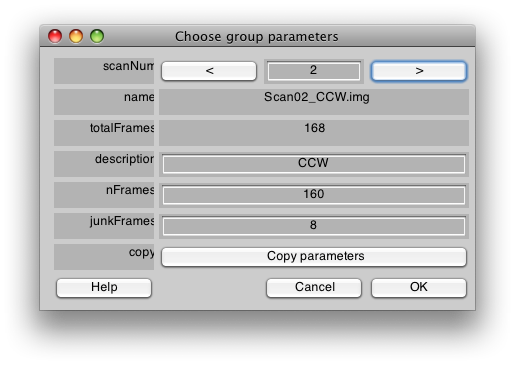
Now, we will add a description string for each scan. For the first scan enter CW. Then press the right arrow next to the scanNum at the top of the dialog to get to the next scan. After you press the right arrow, and you will be editing information for scan 2. Set the description string to CCW and the dialog should look like the following:

Then go through each scan, by pressing the right arrow next to the scanNum, and fill in the correct description. The description is just a name to help you remember what the scan was and could be anything you like (and can later be changed in the mrLoadRet GUI if need be). For these scans, just add either CW/CCW/Expanding/Contracting depending on what the scan .img filename is. When you are done, all scans should have a name and all scans should have junkFrames set to 8. Press OK.

You will get a message that asks if you want to append any notes. Answer no.

You should now be done with mrInit. If you want to check your work, you can use the function groupInfo to confirm that everything got setup correctly. For example, groupInfo alone will give you information about the session that you just entered and should look something like this:

>> groupInfo
========================================
homeDir: /Volumes/drobo/data/anatomy/Retinotopy/
description: Retinotopy Tutorial
operator: Laszlo Jamf subject: Slothrop
magnet: Allegra 3T coil: Siemens birdcage protocol: cbi_ep2d_bold: 
========================================
1: Raw (10 scans) 363.0M

And, the groupInfo on the Raw group should give the following:

>> groupInfo('Raw')
1: CW
   Filename: Scan01_CW.img GroupName: Raw
   junkFrames=[8] totalJunkedFrames=[0]
   voxelSize=[3.0 3.0 3.0] TR=1.5000 Dims: [64 64 27] Volumes=168
2: CCW
   Filename: Scan02_CCW.img GroupName: Raw
   junkFrames=[8] totalJunkedFrames=[0]
   voxelSize=[3.0 3.0 3.0] TR=1.5000 Dims: [64 64 27] Volumes=168
3: Expanding
   Filename: Scan03_EXP.img GroupName: Raw
   junkFrames=[8] totalJunkedFrames=[0]
   voxelSize=[3.0 3.0 3.0] TR=1.5000 Dims: [64 64 27] Volumes=168
4: Contracting
   Filename: Scan04_CON.img GroupName: Raw
   junkFrames=[8] totalJunkedFrames=[0]
   voxelSize=[3.0 3.0 3.0] TR=1.5000 Dims: [64 64 27] Volumes=168
5: CW
   Filename: Scan05_CW.img GroupName: Raw
   junkFrames=[8] totalJunkedFrames=[0]
   voxelSize=[3.0 3.0 3.0] TR=1.5000 Dims: [64 64 27] Volumes=168
6: CCW
   Filename: Scan06_CCW.img GroupName: Raw
   junkFrames=[8] totalJunkedFrames=[0]
   voxelSize=[3.0 3.0 3.0] TR=1.5000 Dims: [64 64 27] Volumes=168
7: Expanding
   Filename: Scan07_EXP.img GroupName: Raw
   junkFrames=[8] totalJunkedFrames=[0]
   voxelSize=[3.0 3.0 3.0] TR=1.5000 Dims: [64 64 27] Volumes=168
8: Contracting
   Filename: Scan08_CON.img GroupName: Raw
   junkFrames=[8] totalJunkedFrames=[0]
   voxelSize=[3.0 3.0 3.0] TR=1.5000 Dims: [64 64 27] Volumes=168
9: CW
   Filename: Scan09_CW.img GroupName: Raw
   junkFrames=[8] totalJunkedFrames=[0]
   voxelSize=[3.0 3.0 3.0] TR=1.5000 Dims: [64 64 27] Volumes=168
10: CCW
   Filename: Scan10_CCW.img GroupName: Raw
   junkFrames=[8] totalJunkedFrames=[0]
   voxelSize=[3.0 3.0 3.0] TR=1.5000 Dims: [64 64 27] Volumes=168

The most important thing is that you got the junkFrames right. If you got something wrong, then you can always change it in the next step, once you run the mrLoadRet viewer. To make changes to the session, use the menu item Edit/Edit mrSession and to change the group information, use Edit/Group/Edit Group

To avoid getting lots of popup warning messages (which you just need to close, set your verbose setting to no):

mrSetPref('verbose','no') 

Now, you are now ready to start the mrLoadRet viewer,

mrLoadRet

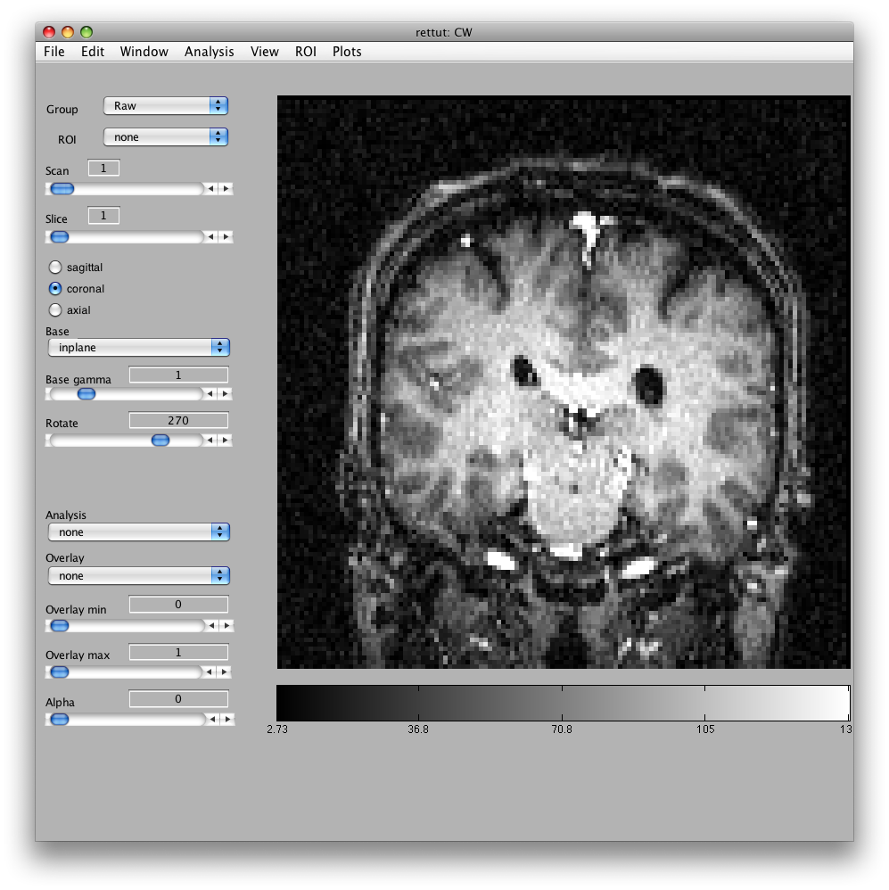
Will bring up a window that looks like the following. Make sure to click on the Coronal/Sagital/Axial radio buttons and play with the slice slider to view whatever slice of the anatomy you want to see:

You may get a couple of warnings about the sform not being set:

If you have verbose set to no, then just ignore. If you get dialog boxes, click Ok to cancel these (and consider following the instructions above or go to Edit→Preferences menu and turn verbose settings to no). They are just warning you that you have not done an alignment yet, which we will do later in the tutorial. Remember to always read the messages printed to the command window if you choose to set verbose warnings to no.

From here, the usual first step is to do motion compensation on the scan. For the purposes of this tutorial, we are going to skip motion compensation (the files provided have already been motion compensated). For more information on how to run motion compensation, please see Motion Compensation. If we had done motion compensation, then all the motion compensated scans would have been moved into a new group called MotionComp and we would make the Averages from the MotionComp group. Instead, we will simply make the Average from the Raw group.

Now, we will average together time series. There are two purposes for doing this. One is to improve the SNR. The other is to remove the effect of the hemodynamic lag. Because we run the rings and the wedges in both directions (e.g. CW and CCW), we can reverse the order of one set of scans (say the CCW) when we average with the CW scans. Now, the hemodynamic lag will make the response lag a few seconds behind the stimulus. We can compensate somewhat for it, by shifting our time series by a few seconds. However, we don't know exactly how long that lag is, but because we are reversing and averaging together, the residual lags we haven't compensated for by shifting will cancel each other out and we get a response that is of average phase between the two scans.

Note that this tutorial is written with a shift forward by 2 frames - the exact shift you need depends on the hemodynamic lag and the difference in starting phase between forward and reverse runs and so shifting forward by 2 frames may not work on other data you collect. It is worth testing out different shifts to see which one gives you the best retinotopy maps. A general guideline is that shifting by -3 to -5 frames (note the negative signs) rather than the +2 in this tutorial works for most cases.

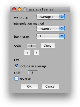
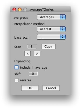
So, to average the wedge scans together, select Analysis/Average Time Series. It should look something like this:

You can ignore the interpolation method and base scan settings. These are only important if you are averaging together scans that come from different slice placements.

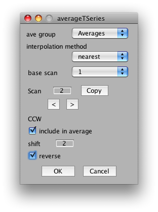
The important settings for us is whether to include the scan in the average, the shift and the reverse flag. We will want to include all CW and CCW scans, set their shift to 2 volumes (approximate compensation for hemodynamic lag) and then reverse all the CCW scans. So, start by setting shift to 2 in the dialog. Now click the right arrow under scan and set Scan 2 to have a shift of 2 and the reverse flag set:

Next, go to scan 3 and unclick it from the average.

And, go through in the same way, setting all CW scans to be included with a shift of 2, all CCW to be included with a shift of 2 and the reverse flag set, and all other scans to not be included.

Click OK. And mrLoadRet will begin to average the scans together.

When it is done, go back and do the same thing again, but this time average together expanding and contracting rings scans setting the shift to 2 volumes and setting all contracting scans to be reversed.

Now, on the main viewer, change the Group drop down to Averages.

It is useful to change the names of the scans we just made to something easier to remember what they are. To do this, go to Edit/Group/Edit Group. The first scan should have the name

Average from Raw of scans: 1   2   5   6   9  10

Change it to

Wedges: Average from Raw of scans: 1   2   5   6   9  10

Change the second scan to

Rings: Average from Raw of scans: 3  4  7  8

And click OK.

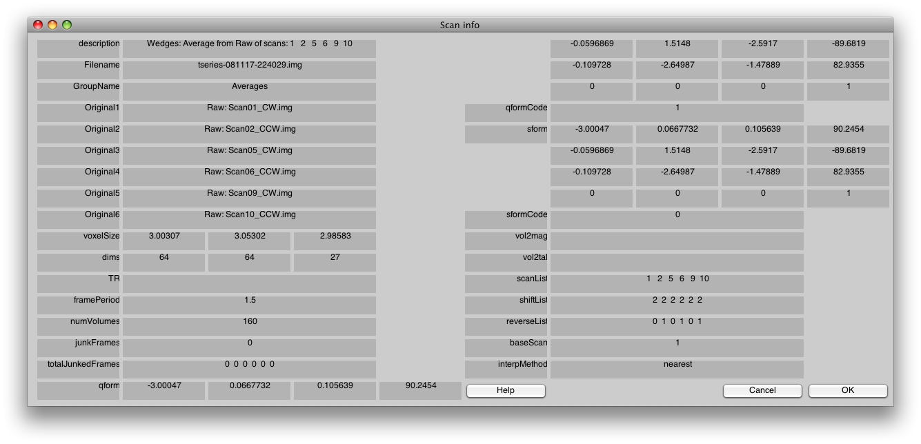
To confirm that you did the averaging right, select Edit/Scan/Info, and you will get a dialog like this:

Pay close attention to the fields scanList, shiftList and reverseList. They tell you how you did your averaging and they should look identical to the above.

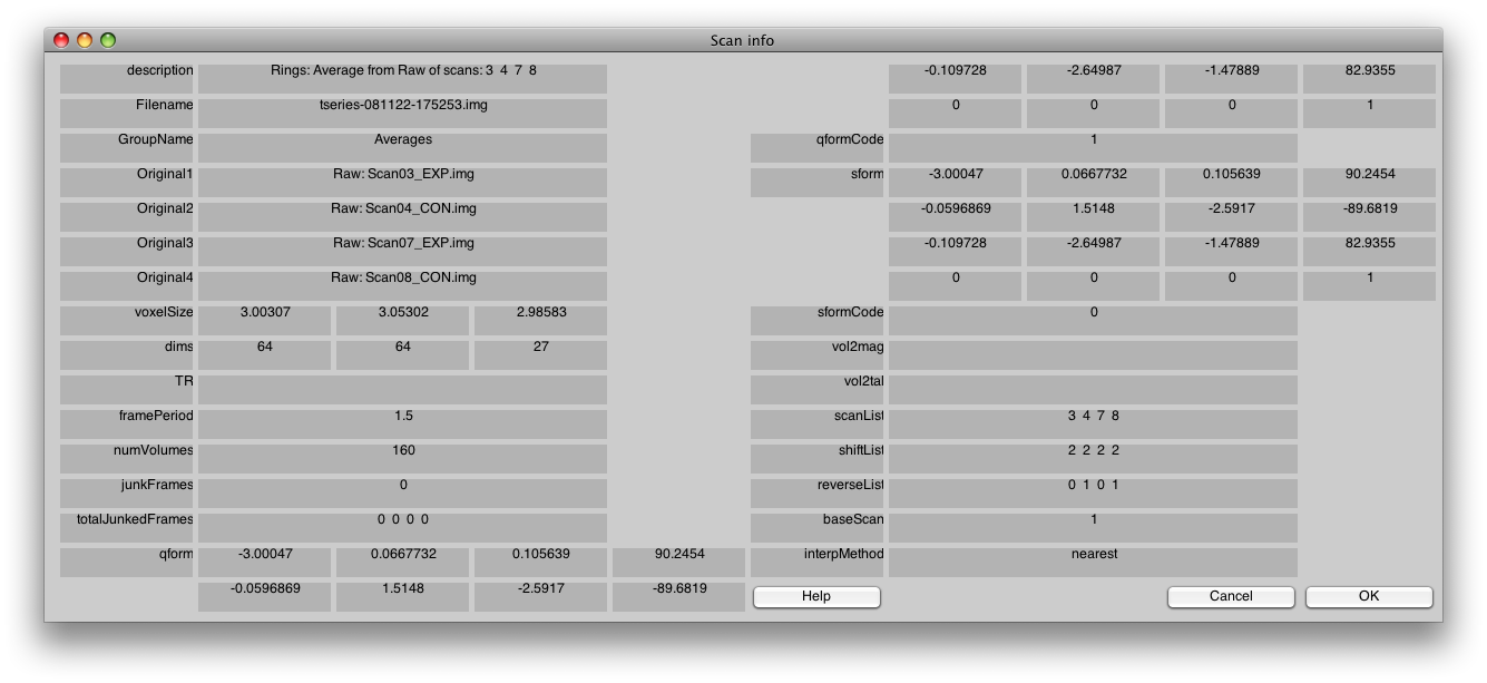
You can also check the rings scan, by sliding the Scan slider on the main viewer to scan 2 and selecting Edit/Scan/Info, and it should look like this:

Now we are ready to run the correlation analysis. Choose the menu item Analysis/Correlation Analysis. For both scans, you will select (re)compute and set the number of cycles to 10. It should look like the following:

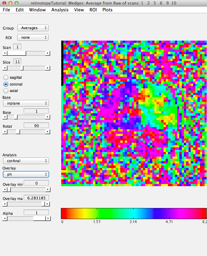
When it has finished running, you should see something like this:

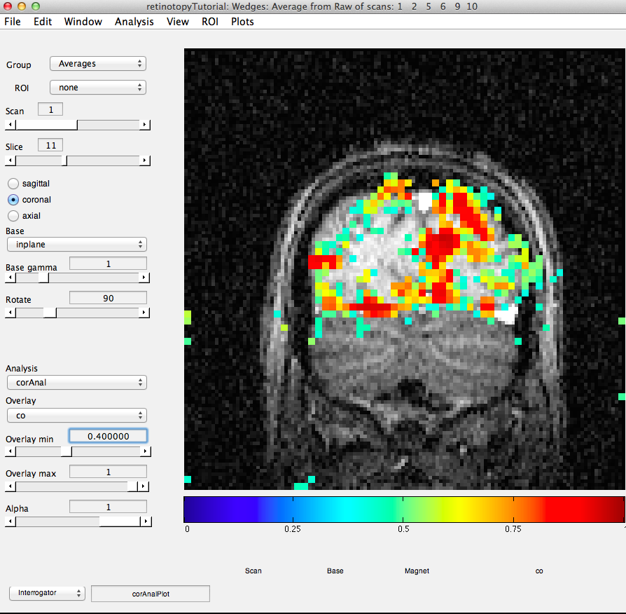
Now, let's try to examine single voxel responses on the map. First, move the Slice slider to Slice 11. Then choose the co Overlay (Coherence). Choose an Overlay min 0f 0.4 so that you are only looking at voxels with a high correlation value. Then turn on the voxel interrogator, by going to Plots/Interrogate Overlay. You should see something like this:

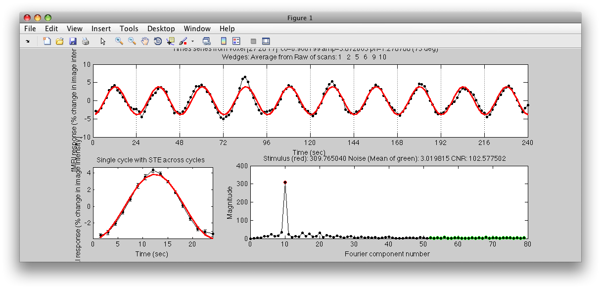
Note the Interrogator drop down in the lower left of the viewer and that it is selected to corAnalPlot. When you move your mouse over the image it should now turn into a giant cross-hairs. Choose one of the voxels (the example below is voxel [27 28 11]) with the darkest red color and click. After a moment, you should see a figure like this:

Looks very well modulated at the stimulus frequency! Contrast-to-noise ratio (i.e. the magnitude of the response at the task frequency (marked in red in the lower right graph, divided by the mean of the points marked in green) is over a 100-to-1.

Now set the Overlay min slider back to 0 (just for visualization purposes later in the tutorial).

Now we will run the alignment so that we can view the data on a flat surface. Start up mrAlign:

mrAlign

From File/Load Destination (Volume) go and find the volume anatomy (Anatomy/volume.img) and load it. From the File/Load Source (Inplane) go and find the inplane anatomy (Anatomy/inplane.img) and load it.

Under Compute Alignment, choose Initialize Alignment from Header.

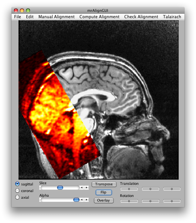
Now set the slice slider to somewhere in the middle and click Transpose and Flip and you should see something like this:

You can run a full alignment by going into the Compute Alignment menu, but for this example the Alignment from Header has been cooked to be perfect. (Normally, this won't be the case, check the mrAlign documentation for more info on all the parameters you can set for real alignments).

So, instead just go to File/Save Alignment and save the alignment. This saves the alignment between your inplanes and the reference volume anatomy in the header (sform field) of the nifti inplane.img file.

Now we need to align the scans with this inplane. We can do that by first going to File/Reload Source as Destination to set the inplanes as the slices that we are aligning to.

Next File/Load Source (inplane), and go to Raw/TSeries and select any one of the Scan files. Shortly, a dialog will come up and you can select the mean image to display (since the epi images are a sequence of images, you have to choose either to show the mean or a particular time frame). Note that on some systems this dialog may pop-up *below* the mrAlign viewer. If this happens just move the mrAlign viewer until you see the dialog.

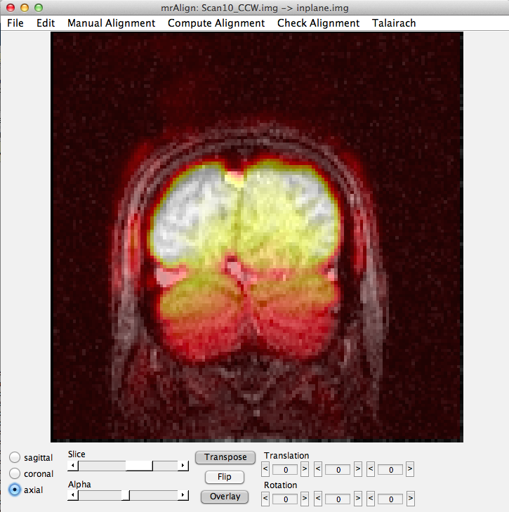
Now select Compute Alignment/Initialize Alignment from Header. Since the scan images were taken during the same session as the inplanes, the initial alignment in the header should be perfect (unless the subject moved their head). Click the axial button, the flip button and select a middle slice and set the alpha to about 50%, and you should see something like this:

Now you are ready to export the alignment to the mrLoadRet Session. Go to File/Export/Export to mrLoadRet-4.5 and click yes on the dialog that comes up, then you will be given the option of what groups to export to. You should export to all groups and press OK.

Quit out of mrAlign, you are done with alignment.

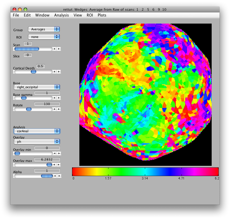
Now, load the flat patch of the right occipital cortex as your base anatomy. Go to File/Base Anatomy/Load and load the file right_occipital.img. If you go back to viewing the ph overlay on Scan 1, you should see something like this:

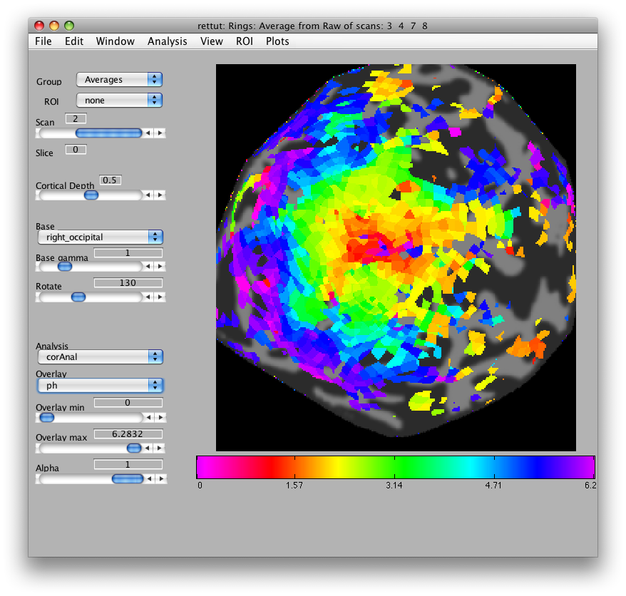
This is the phase map for the wedges, so the color represents the polar angle of the visual field. We can switch to scan 2 and look at the eccentricity map as well. To do that switch the slider to Scan 2.

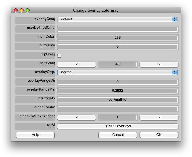
There are a few visualization settings that are also useful to play around with now. One, is to not show voxels that have low coherence with the stimulus. You can do that by choosing the co Overlay in the drop down menu on the main window, and then setting the Overlay min to say 0.3. Now switch back to the ph Overlay and you should see only voxels with high coherence with the stimulus. You can also change the colormap if you like, to do that go to Edit/Overlay/Edit Overlay and you will get a dialog like the following:

If you shiftCmap by 48, you should get a map that looks like this:

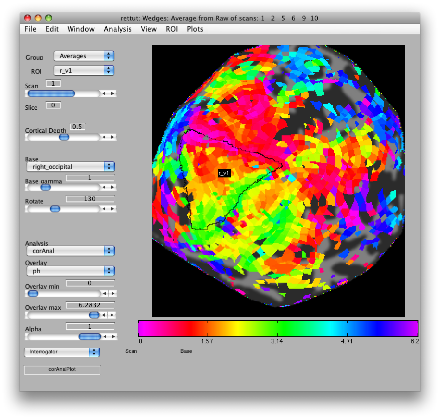
Now, looking at the right_occipital flat map, set the Overlay min to about 0.2 co value and switch back to the ph Overlay. The red/pink points are the lower vertical meridian and the greenish points are the upper vertical meridian. V1 covers the whole contralateral hemifield, so we start by marking off an ROI the spans these two meridians. Go to ROI/Create/Polygon and then give the ROI the name r_v1. Then place points to mark off the area shown below. When you are done marking off the area, double-click:

Note that if you are unhappy with the ROI drawing tool (e.g. it is very slow), you can change how it works in Edit/Preference/roiPolygonMethod.

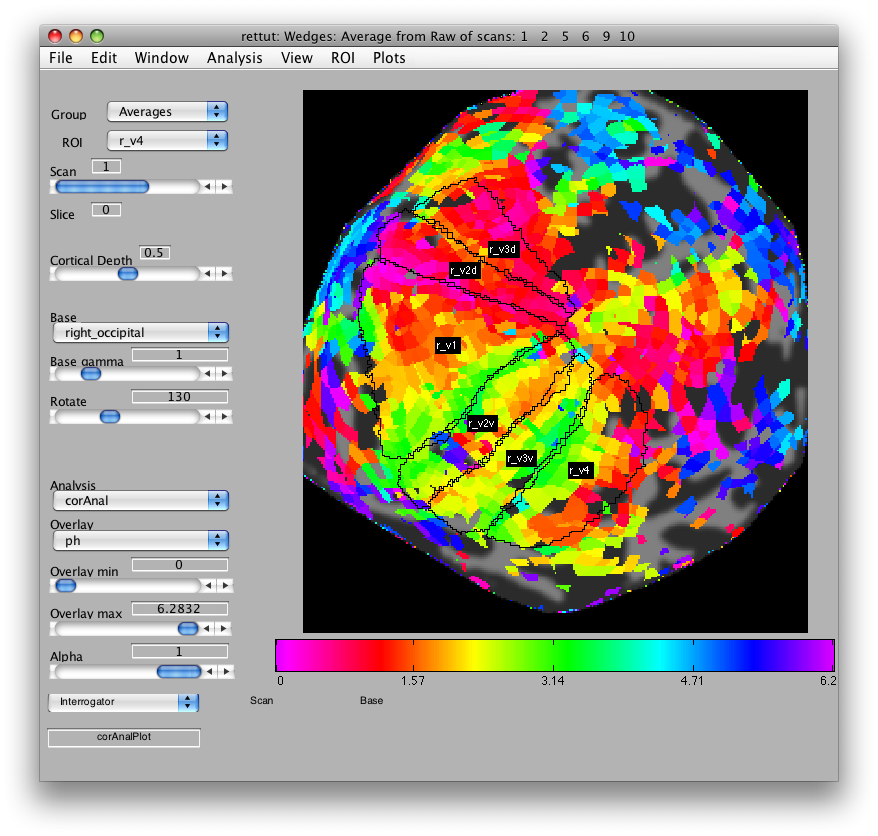
Now, you can draw r_v2d using the same method, by drawing from the lower vertical meridian to the horizontal meridian (yellowish color) and then r_v3d as the horizontal meridian to the lower vertical meridian. Then, similarly for the ventral parts of v2 and v3, you draw from the upper vertical meridian (green) to the horizontal meridian (yellow) and back again. Finally, we draw (though there is some controversy on this issue) V4 as the full hemifield map below v3v. Of course, there are many other visual areas that you can be able to define. For more information on other areas we routinely define, see Larsson & Heeger (2006) and Schluppeck, Glimcher & Heeger (2005) and references therein. and It should look something like:

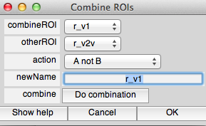
If you want to make sure that ROIs do not overlay each other, you can use the combine tool in ROI/Combine. For instance if you want to make sure that r_v1 has no voxels from r_v2d you would set up the dialog like this:

and press Do combination.

You'd then get a dialog box asking how you want to deal with the non-unique roi name. Check the replace box:

Hitting the OK button will perform the action and subsequently close the “Combine ROIs” dialog box. The “Do Combination” button will perform the action and keep the dialog box open, as it is usually the case there are many rois you want to combine.

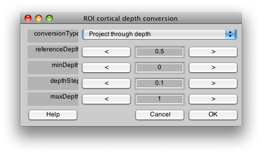
Finally, you may want to extend your ROIs through the cortical depth. Note that by default you are looking at the midcortical depth (See Cortical Depth slider on the main viewer). If you want your ROIs to extend through the gray matter, you can ROI/Convert/Convert cortical depth. You want to Project through depth, and then starting at your current depth (0.5) copy the ROI through the whole gray matter. So you set referenceDepth to 0.5 and then starting at 0 (minDepth) go in increments of 0.1 (depthStep) until reaching the maxDepth of 1, adding voxels that are in the same location to the ROI. Be aware that if you extend too far with your ROI, you may start to cross sulcal boundaries, so use this tool carefully. Also, this tool will only convert voxels if they exist in the currently displayed flat map - so if you want to do rois on the other hemisphere, you will have to switch to the other hemispheres flatmap and convert those rois separately:

When you are done, save your ROIs from the File/ROI/Save all menu item.

Ok! That's it. When you quit through the menu item, you might find that it takes a bit of time to close. This is because mrLoadRet is saving your settings into a file called mrLastView.mat so that when you start again everything will be back in the same place you left it. If you don't want to save your settings, you can always type mrQuit(0) at the command line and mrLoadRet will close without saving. Or, the next time you run, you can run mrLoadRet with mrLoadRet([]) and it will run without loading the mrLastView.mat file. Be aware that until you explicitly save ROIs through the File menu, the ROIs only exist in the mrLastView.mat. Your correlation analysis and the averaging on the other hand has already been saved to disk. You can always reload the Analysis from the File/Analysis/Load menu item.

One last thing that is worth mentioning here. If you don't like all the dialog box warnings, you should set Edit/Preferences/Verbose to “No”. This will print all warnings and errors to the Matlab buffer, so be sure to check there to make sure you don't miss important messages. You should always take note of messages in the console and get used to looking at that output and knowing what it means and what to expect. Also, if the code crashes at some point, it may put you into the Matlab debug mode, that looks like this:

K>>

If you see this happening, you should note what error occurred and then get out of debug mode by typing

K>> dbquit

Note that you can reduce the number of such occurrences by using the GUI in the way that it is intended. Generally, take it slow and be methodical rather than freaking out and clicking on everything in sight! You should be especially careful to use the File/Quit menu item from the main GUI to close MLR since that will guarantee that the next time you load the viewer, you will return to the same state of the viewer including all the same loaded Anatomies, ROIs and Analyses.

-jg.