Table of Contents
mrTools Overview
mrTools provides a set of Matlab tools to analyze fMRI data. It can do basic analyses like correlation analyses used in retinotopy experiments, event-related, population RF and GLM analyses. It can display the results of analyses on inplane anatomies, flat maps and surfaces. It is designed to make it easy to write your own script and programs in Matlab to analyze your data.
There are tutorials available for doing retinotopy, pRF, event-related analysis, classification and GLM.
Download
You can access an up-to-date read-only archive of mrTools using subversion:
svn checkout https://cbi.nyu.edu/svn/mrTools/trunk mrTools
Once you have used checkout to get the repository, you can get updates whenever you want to by doing:
svn update
The current directory must be 'mrTools', when you want to update.
See the commit logs for what has changed recently.
We recommend using subversion (see here for a quick primer) if at all possible (so that you can easily stay on top of the many improvements to the code we continue to make). Mac OS 10.5-7 comes with subversion preinstalled. The latest versions of Mac OS 10.8 (Mountain Lion) does not have svn preinstalled. You can install svn by installing the latest Xcode (make sure that you have checked the option to install the command line tools to get svn - if you already have Xcode installed, but svn is not installed, go to Xcode > Preferences > Downloads > Command Line Tools > Install). You will also need to have Xcode installed if you need to recompile mgl. For non-mac users, you can install svn directly from the subversion website. If you are really unable to get subversion, you can download mrTools.tar.gz which contains a current version of the code. It should just open by clicking on it. If not, from a command line, you should be able to do:
gunzip mrtools.tar.gz
tar xfv mrtools.tar
Once you have downloaded, see Getting Started for installation instructions.
Switching from previous svn repository
If you have an old svn repository that you downloaded from http://yoyodyne.cns.nyu.edu/svn/mrTools/trunk, then you can switch to the new repository by cd'ing to your mrTools directory and running:
svn switch --relocate http://yoyodyne.cns.nyu.edu/svn/mrTools/trunk http://cbi.nyu.edu/svn/mrTools/trunk
Problems downloading with SVN
If you have problems downloading with svn because your institution has a proxy server, you might have to let subversion know about it. Have a look at download_with_proxy-server for details on how to set this up.
Getting Started
Add mrTools to your matlab path
At the Matlab prompt, type
addpath(genpath('/folderWhereYouInstalled/mrTools'))
Where folderWhereYouInstalled should be replaced with the name of the folder in which you have downloaded the svn or cvs repository.
Quick overview
The best way to get started using MLR is to go through the Retinotopy Tutorial. In the tutorial you will learn the basic steps of setting up an MLR session which are as follows:
- Make the directory structure for MLR.
- Anatomy contains the inplane and any other anatomy file used by MLR.
- Raw/TSeries contains the epi images of each scan.
- Etc Contains supplementary files like stimulus timing files.
- Run mrInit or mrInitRet.
- Run mrAlign and align your inplane anatomy to your “canonical” volume anatomy. Then align your epi images to the inplane anatomy and export to mrLoadRet-4.5.
- Run Motion Compensation.
Note: To run mrTools, you need the following MATLAB toolboxes: Optimization, Statistics and Image Processing.
Compiling MEX files
MEX files (Matlab C code) for several functions are pre-compiled to improve performance – you should not need to do anything if you want to use them on the following platforms: MacIntel (.mexmaci), PowerPC Mac (.mexmac) and 64-bit Linux (.mexa64). The following is a list of the mex files used in MLR:
- mrAlign/regHistogram.c
- mrUtilities/ImageProcessing/myCinterp3.c
- mrUtilities/MatlabUtilities/mrDisp.c
- mrUtilities/mrFlatMesh/assignToNearest.c
- mrUtilities/mrFlatMesh/dijkstra.cpp
If you have trouble with any of these functions, you may want to recompile them. This can be done by cd'ing to the directory where the function lives, and typing (e.g.):
mex mrDisp.c
Note that to compile these functions on a Mac you will need to have Xcode installed on your computer. On other platforms you will need to have the gcc compiler.
If compilation fails it may be because we use some c++ syntax in the files (comments that begin with // and variables not declared at the top of functions) and gcc is interpreting the .c file as ANSI c. You can override the ANSI c compilation and force a c++ compilation on most systems by doing:
mex CC=g++ mrDisp.c
If you need to re-compile any mex functions for a 64bit platform, here are some things you should watch out for:
- to compile MEX files (usually .c or .cpp) on Matlab version 7.3 and later, you should make sure you have GCC version 4.0 or later installed. Some *nix distributions still have GCC3.3, which will not work
- if the c/c++ code includes sparse matrix operations (like e.g. dijkstra.cpp) you should be aware that The Mathworks has changed indeces into these matrices from type int to mwIndex
- to make use of larger array sizes allowed by 64 bits you need to compile the mex files with the option -largeArrayDims , e.g.
>> mex -largeArrayDims dijkstra.cpp
Printing this manual
If you wish to print out this manual, you can view it as a single page and print from there.
Mailing List
If you want to subscribe to an email list which will make (very infrequent) announcements about major changes to mrTools, you can do so from http://cbi.nyu.edu/mailman/listinfo/mrtools-announce. Note that this is a moderated email list to which you will not be able to make posts, only receive announcements.
Retinotopy Tutorial
This tutorial shows you how to run a retinotopy analysis with mrLoadRet. It is a good place to start if you are just learning how to use mrLoadRet.
Overview
- Download the tutorial files
- The stimuli used in the experiment
- Make the directory structure for mrLoadRet and move the files into the correct locations
- Run mrInit to initialize the session
- Run the Motion Compensation
- Average wedge and ring scans together
- Run the correlation analysis
- Use mrAlign to align the 2D inplane anatomy to the 3D volume anatomy
- View the results on a flattened representation of occipital cortex
- Draw the visual area ROIs
1. Download files
You can download the tutorial files from:
Note that this is a rather big file, approximately 300MB.
The files are provided as a tar/zip file. In Mac OS X you should be able to just click to open the files in the Finder. Otherwise, you can go to a terminal and do:
gunzip retinotopyTutorial.tar.gz
tar xvf retinotopyTutorial.tar
We provide you with a set of 10 functional scans, an inplane anatomy file, a high-resolution T1-weighted volume anatomy used for alignment and a flat map of the right occipital cortex to visualize the results on.
The functional scans include 6 rotating wedge runs (3 CW and 3 CCW rotations) and 4 expanding and contracting ring runs (2 expanding and 2 contracting). Each run is 168 volumes long (a volume was acquired every 1.5 seconds). The first 8 volumes will be thrown out to allow hemodynamic response and longitudinal magnetization to reach steady state. The data has already been motion compensated (since this step takes quite a bit of time to run).
From here, all the directions will be for commands to run under Matlab. It is assumed that you have properly set up mrTools using the directions under Getting Started.
2. Stimuli
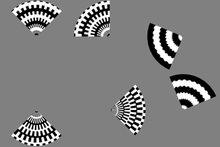
The visual stimuli were run using the mglDoRetinotopy command in the mgl library. A CCW wedge run looks something like the following (though the animating gif probably doesn't play at the right speed – each cycle should take 24 seconds).
The rings stimuli look something like this:
3. mrLoadRet directory structure
Now that you have the raw image files, you need to make the directory structure for mrLoadRet and copy your files into the correct directories. (Note that this does not have to be done in Matlab, it can be done from the command line or from the Finder or from a shell script that is customized for the file types at your site).
- Start up Matlab and change directories into the downloaded tutorial data directory
cd retinotopyTutorial
- Now make a directory for the anatomy files and move the anatomies into that directory.
  mkdir Anatomy
  movefile inplane.* Anatomy
  movefile volume.* Anatomy
  movefile right_occipital.* Anatomy
- Now make the directory to hold your raw time series (i.e. the epi scans with your data), and move the scan files into that directory
  mkdir Raw
  mkdir Raw/TSeries
  movefile Scan* Raw/TSeries
You should now have two top level directories (Anatomy and Raw) and all the files should have been moved into one of the sub-directories:
>> ls
Anatomy/     Raw/
4. mrInit
Now you are ready to run mrInit which will setup your mrLoadRet session:
mrInit
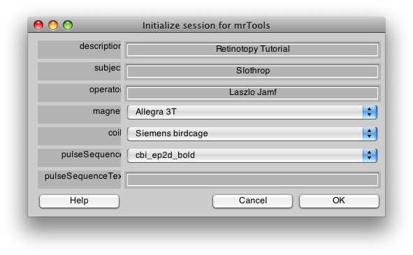
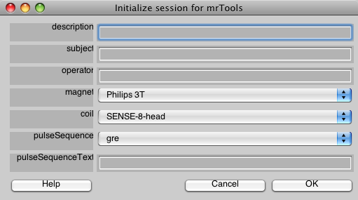
You will first see a dialog like the following. Go ahead and fill in the fields to match what is shown here. This is information about the scan, it is used only for documentation, so you will usually fill in the fields appropriately for the scan you are running. Also, if you are using a different magnet and coil than the one at NYU, you can see the section mrInit on how to customize this dialog to your site. Finally, you may always change this information later, from the mrLoadRet GUI. When you are done, click OK.
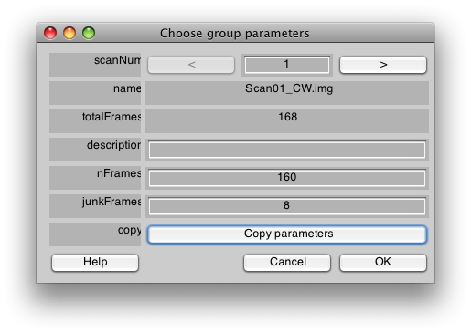
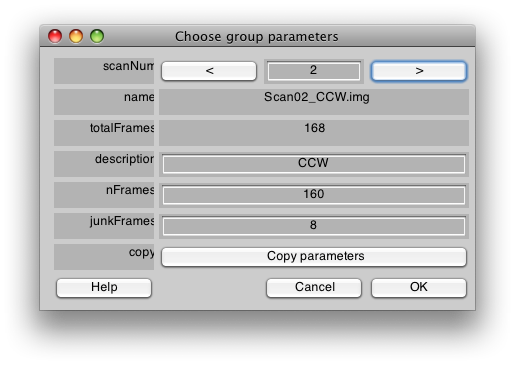
Now you will get a dialog to set the parameters for each scan in the session. For these we are going to give a name to each scan (either CW, CCW, Expanding, or Contracting), and set the number of junkFrames to 8. The junkFrames mean to throw out the first 8 frames of the scan, we do this because we always take an extra half cycle of the stimulus (16 volumes per cycle), to allow both the longitudanal magnetization and hemodynamic response to reach steady-state. Let's start by setting all the scans to have junkFrames of 8. We can do this by putting 8 into the junkFrames field and then pressing “Copy parameters”:
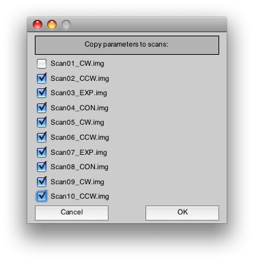
Select all the rest of the scans. This is the quickest way to copy the junkFrames parameter to all of those scans. Press Ok.
Now, we will add a description string for each scan. For the first scan enter CW. Then press the right arrow next to the scanNum at the top of the dialog to get to the next scan. After you press the right arrow, and you will be editing information for scan 2. Set the description string to CCW and the dialog should look like the following:
Then go through each scan, by pressing the right arrow next to the scanNum, and fill in the correct description. The description is just a name to help you remember what the scan was and could be anything you like (and can later be changed in the mrLoadRet GUI if need be). For these scans, just add either CW/CCW/Expanding/Contracting depending on what the scan .img filename is. When you are done, all scans should have a name and all scans should have junkFrames set to 8. Press OK.
You will get a message that asks if you want to append any notes. Answer no.
You should now be done with mrInit. If you want to check your work, you can use the function groupInfo to confirm that everything got setup correctly. For example, groupInfo alone will give you information about the session that you just entered and should look something like this:
>> groupInfo
========================================
homeDir: /Volumes/drobo/data/anatomy/Retinotopy/
description: Retinotopy Tutorial
operator: Laszlo Jamf subject: Slothrop
magnet: Allegra 3T coil: Siemens birdcage protocol: cbi_ep2d_bold:
========================================
1: Raw (10 scans) 363.0M
And, the groupInfo on the Raw group should give the following:
>> groupInfo('Raw')
1: CW
   Filename: Scan01_CW.img GroupName: Raw
   junkFrames=[8] totalJunkedFrames=[0]
   voxelSize=[3.0 3.0 3.0] TR=1.5000 Dims: [64 64 27] Volumes=168
2: CCW
   Filename: Scan02_CCW.img GroupName: Raw
   junkFrames=[8] totalJunkedFrames=[0]
   voxelSize=[3.0 3.0 3.0] TR=1.5000 Dims: [64 64 27] Volumes=168
3: Expanding
   Filename: Scan03_EXP.img GroupName: Raw
   junkFrames=[8] totalJunkedFrames=[0]
   voxelSize=[3.0 3.0 3.0] TR=1.5000 Dims: [64 64 27] Volumes=168
4: Contracting
   Filename: Scan04_CON.img GroupName: Raw
   junkFrames=[8] totalJunkedFrames=[0]
   voxelSize=[3.0 3.0 3.0] TR=1.5000 Dims: [64 64 27] Volumes=168
5: CW
   Filename: Scan05_CW.img GroupName: Raw
   junkFrames=[8] totalJunkedFrames=[0]
   voxelSize=[3.0 3.0 3.0] TR=1.5000 Dims: [64 64 27] Volumes=168
6: CCW
   Filename: Scan06_CCW.img GroupName: Raw
   junkFrames=[8] totalJunkedFrames=[0]
   voxelSize=[3.0 3.0 3.0] TR=1.5000 Dims: [64 64 27] Volumes=168
7: Expanding
   Filename: Scan07_EXP.img GroupName: Raw
   junkFrames=[8] totalJunkedFrames=[0]
   voxelSize=[3.0 3.0 3.0] TR=1.5000 Dims: [64 64 27] Volumes=168
8: Contracting
   Filename: Scan08_CON.img GroupName: Raw
   junkFrames=[8] totalJunkedFrames=[0]
   voxelSize=[3.0 3.0 3.0] TR=1.5000 Dims: [64 64 27] Volumes=168
9: CW
   Filename: Scan09_CW.img GroupName: Raw
   junkFrames=[8] totalJunkedFrames=[0]
   voxelSize=[3.0 3.0 3.0] TR=1.5000 Dims: [64 64 27] Volumes=168
10: CCW
   Filename: Scan10_CCW.img GroupName: Raw
   junkFrames=[8] totalJunkedFrames=[0]
   voxelSize=[3.0 3.0 3.0] TR=1.5000 Dims: [64 64 27] Volumes=168
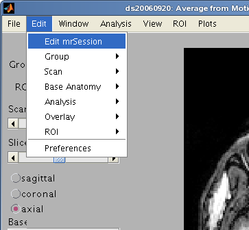
The most important thing is that you got the junkFrames right. If you got something wrong, then you can always change it in the next step, once you run the mrLoadRet viewer. To make changes to the session, use the menu item Edit/Edit mrSession and to change the group information, use Edit/Group/Edit Group
5. Motion Compensation
You are now ready to start the mrLoadRet viewer:
mrLoadRet
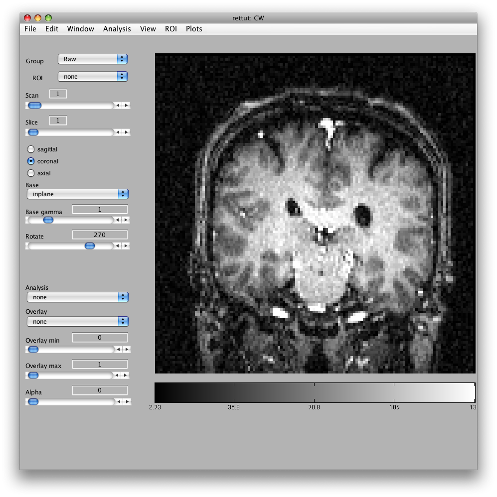
Will bring up a window that looks like the following. Make sure to click on the Coronal/Sagital/Axial radio buttons and play with the slice slider to view whatever slice of the anatomy you want to see:
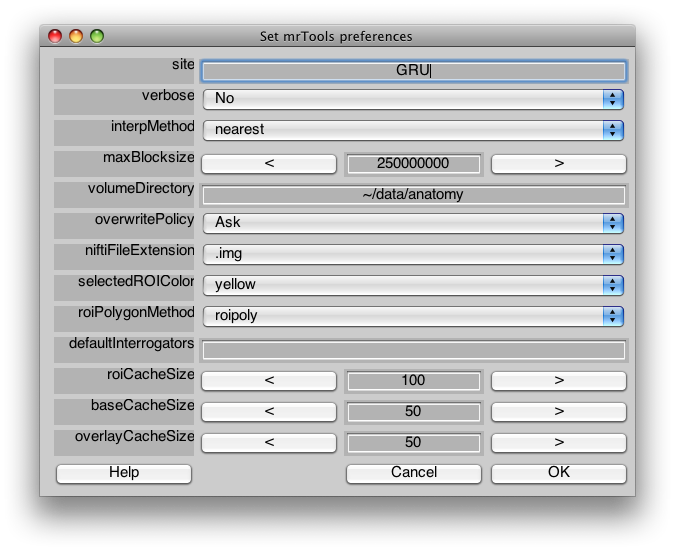
You may get a couple of warnings about the sform not being set. Click Ok to cancel these. They are just warning you that you have not done an alignment yet, which we will do later in the tutorial. If you prefer not to get pop-up warnings and wait bars and instead would like to have these messages only printed out to the Matlab command window, you should set the verbose preference (Edit→Preferences menu) to No (remember to always read the messages printed to the command window if you choose this setting!)
From here, the usual first step is to do motion compensation on the scan. For the purposes of this tutorial, we are going to skip motion compensation (the files provided have already been motion compensated). For more information on how to run motion compensation, please see Motion Compensation. If we had done motion compensation, then all the motion compensated scans would have been moved into a new group called MotionComp and we would make the Averages from the MotionComp group. Instead, we will simply make the Average from the Raw group.
6. Average time series
Now, we will average together time series. There are two purposes for doing this. One is to improve the SNR. The other is to remove the effect of the hemodynamic lag. Because we run the rings and the wedges in both directions (e.g. CW and CCW), we can reverse the order of one set of scans (say the CCW) when we average with the CW scans. Now, the hemodynamic lag will make the response lag a few seconds behind the stimulus. We can compensate somewhat for it, by shifting our time series by a few seconds. However, we don't know exactly how long that lag is, but because we are reversing and averaging together, the residual lags we haven't compensated for by shifting will cancel each other out and we get a response that is of average phase between the two scans.
Note that this tutorial is written with a shift forward by 2 frames - the exact shift you need depends on the hemodynamic lag and the difference in starting phase between forward and reverse runs and so shifting forward by 2 frames may not work on other data you collect. It is worth testing out different shifts to see which one gives you the best retinotopy maps. A general guideline is that shifting by -3 to -5 frames (note the negative signs) rather than the +2 in this tutorial works for most cases.
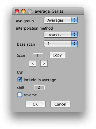
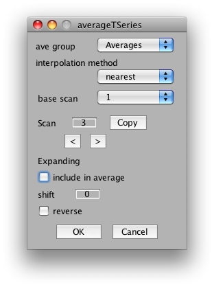
So, to average the wedge scans together, select Analysis/Average Time Series. It should look something like this:
You can ignore the interpolation method and base scan settings. These are only important if you are averaging together scans that come from different slice placements.
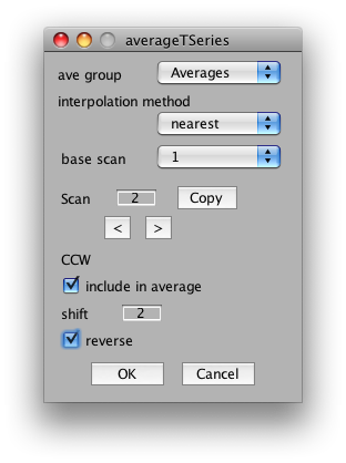
The important settings for us is whether to include the scan in the average, the shift and the reverse flag. We will want to include all CW and CCW scans, set their shift to 2 volumes (approximate compensation for hemodynamic lag) and then reverse all the CCW scans. So, start by setting shift to 2 in the dialog. Now click the right arrow under scan and set Scan 2 to have a shift of 2 and the reverse flag set:
Next, go to scan 3 and unclick it from the average.
And, go through in the same way, setting all CW scans to be included with a shift of 2, all CCW to be included with a shift of 2 and the reverse flag set, and all other scans to not be included.
Click OK. And mrLoadRet will begin to average the scans together.
When it is done, go back and do the same thing again, but this time average together expanding and contracting rings scans setting the shift to 2 volumes and setting all contracting scans to be reversed.
Now, on the main viewer, change the Group drop down to Averages.
It is useful to change the names of the scans we just made to something easier to remember what they are. To do this, go to Edit/Group/Edit Group. The first scan should have the name
Average from Raw of scans: 1 2 5 6 9 10
Change it to
Wedges: Average from Raw of scans: 1 2 5 6 9 10
Change the second scan to
Rings: Average from Raw of scans: 3 4 7 8
And click OK.
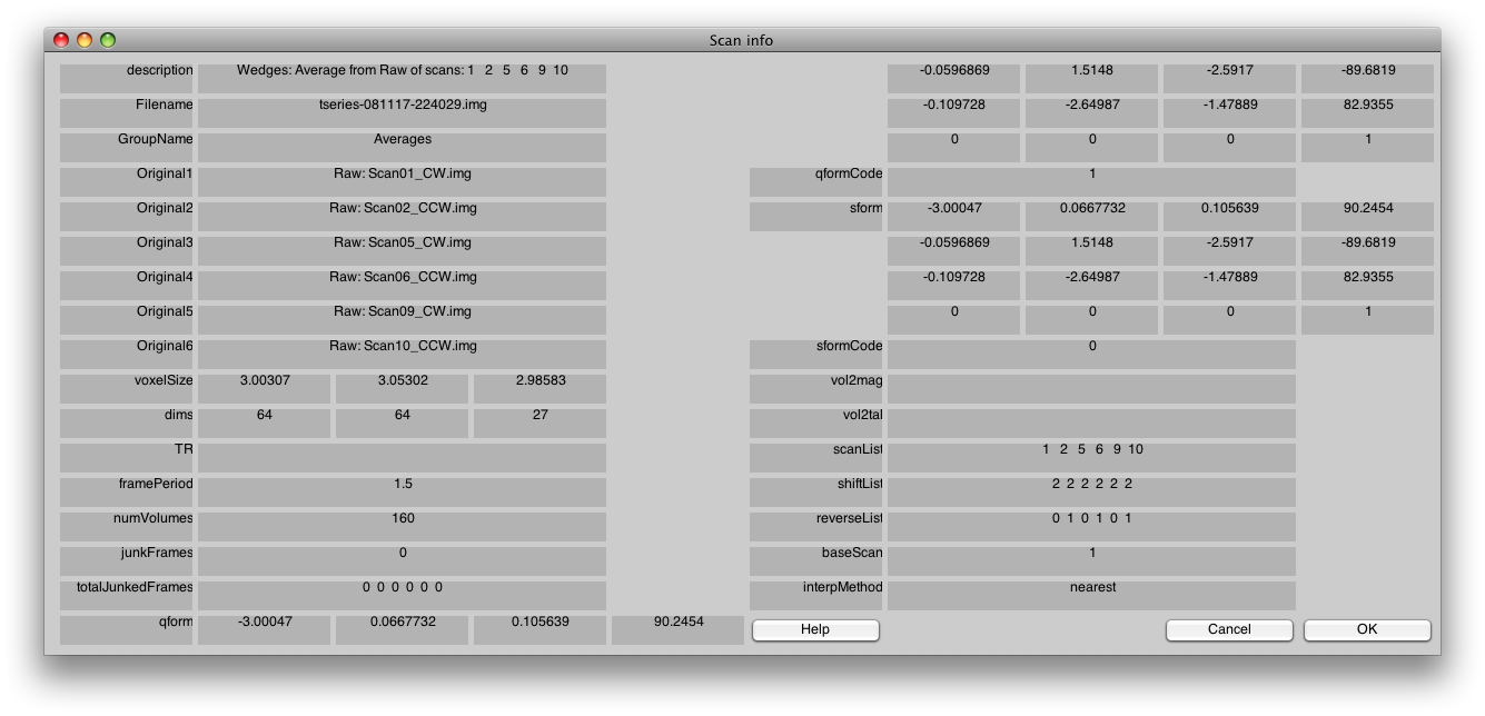
To confirm that you did the averaging right, select Edit/Scan/Info, and you will get a dialog like this:
Pay close attention to the fields scanList, shiftList and reverseList. They tell you how you did your averaging and they should look identical to the above.
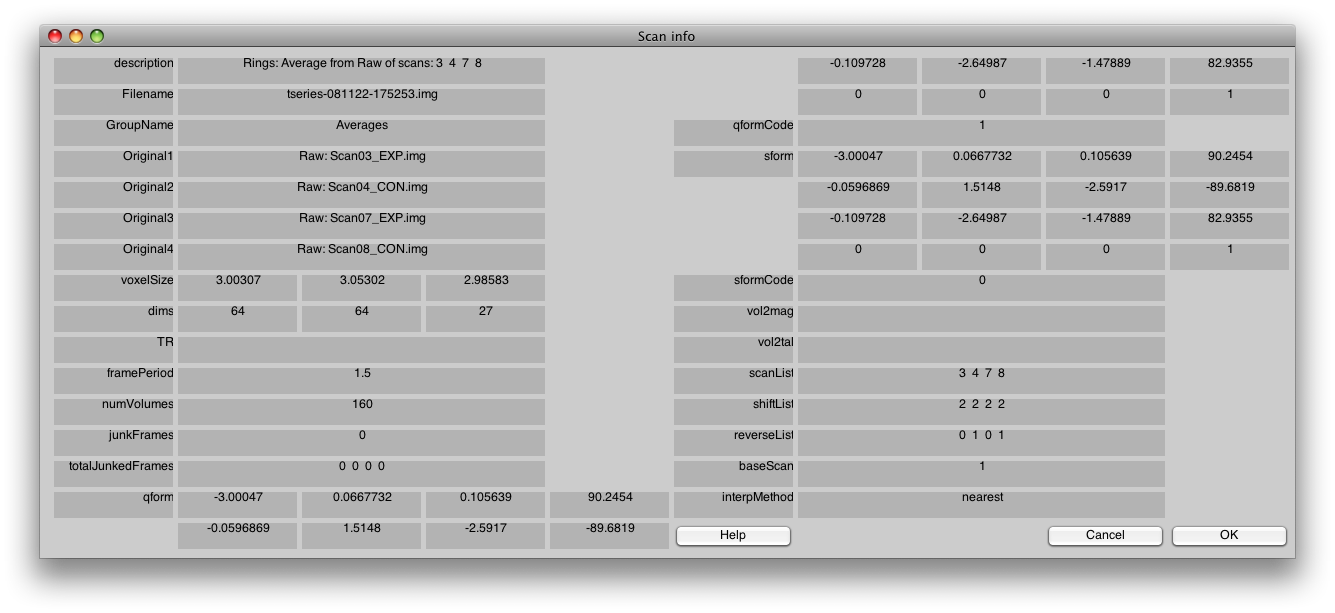
You can also check the rings scan, by sliding the Scan slider on the main viewer to scan 2 and selecting Edit/Scan/Info, and it should look like this:
7. Correlation analysis
Now we are ready to run the correlation analysis. Choose the menu item Analysis/Correlation Analysis. For both scans, you will select (re)compute and set the number of cycles to 10. It should look like the following:
When it has finished running, you should see something like this:
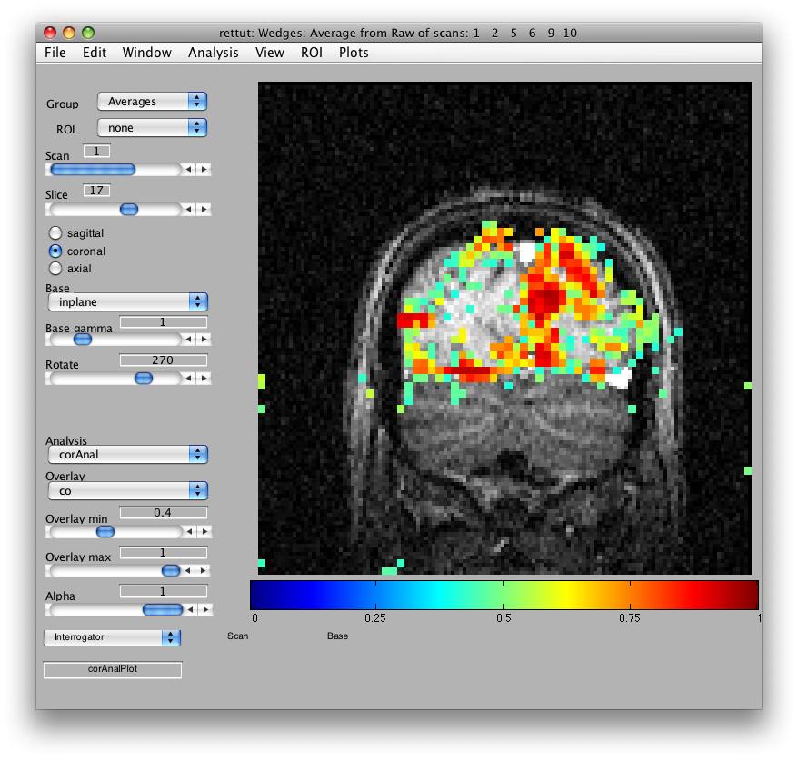
Now, let's try to examine single voxel responses on the map. First, move the Slice slider to Slice 17. Then choose the co Overlay (Coherence). Choose an Overlay min 0f 0.4 so that you are only looking at voxels with a high correlation value. Then turn on the voxel interrogator, by going to Plots/Interrogate Overlay. You should see something like this:
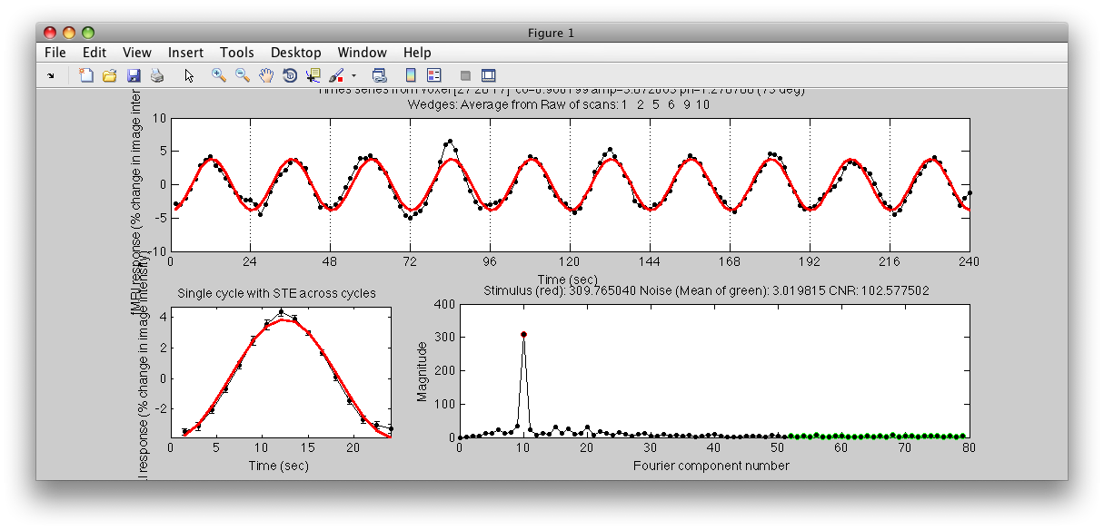
Note the Interrogator drop down in the lower left of the viewer and that it is selected to corAnalPlot. When you move your mouse over the image it should now turn into a giant cross-hairs. Choose one of the voxels (the example below is voxel [27 28 17]) with the darkest red color and click. After a moment, you should see a figure like this:
Looks very well modulated at the stimulus frequency! Contrast-to-noise ratio (i.e. the magnitude of the response at the task frequency (marked in red in the lower right graph, divided by the mean of the points marked in green) is over a 100-to-1.
8. Run Alignment
Now we will run the alignment so that we can view the data on a flat surface. Start up mrAlign:
mrAlign
From File/Load Destination (Volume) go and find the volume anatomy (Anatomy/volume.img) and load it. From the File/Load Source (Inplane) go and find the inplane anatomy (Anatomy/inplane.img) and load it.
Under Compute Alignment, choose Initialize Alignment from Header.
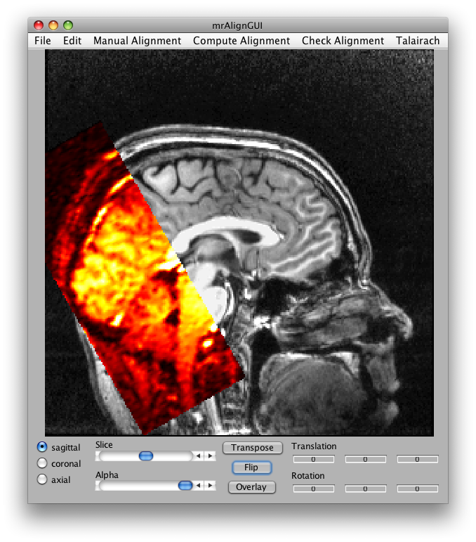
Now set the slice slider to somewhere in the middle and click Transpose and Flip and you should see something like this:
You can run a full alignment by going into the Compute Alignment menu, but for this example the Alignment from Header has been cooked to be perfect. (Normally, this won't be the case, check the mrAlign documentation for more info on all the parameters you can set for real alignments).
So, instead just go to File/Save Alignment and save the alignment. This saves the alignment between your inplanes and the reference volume anatomy in the header (sform field) of the nifti inplane.img file.
Now we need to align the scans with this inplane. We can do that by first going to File/Reload Source as Destination to set the inplanes as the slices that we are aligning to.
Next File/Load Source (inplane), and go to Raw/TSeries and select any one of the Scan files. Shortly, a dialog will come up and you can select the mean image to display (since the epi images are a sequence of images, you have to choose either to show the mean or a particular time frame). Note that on some systems this dialog may pop-up *below* the mrAlign viewer. If this happens just move the mrAlign viewer until you see the dialog.
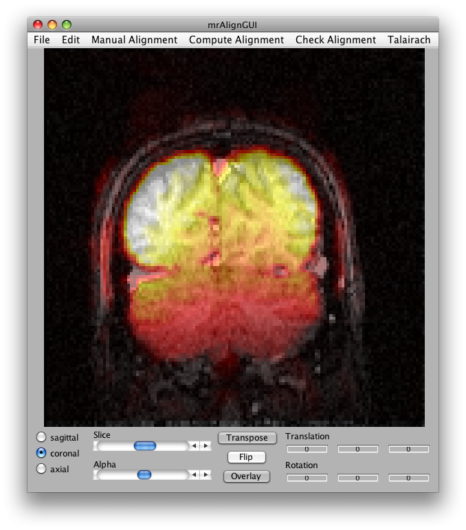
Now select Compute Alignment/Initialize Alignment from Header. Since the scan images were taken during the same session as the inplanes, the initial alignment in the header should be perfect (unless the subject moved their head). Click the coronal button, the flip button and select a middle slice and set the alpha to about 50%, and you should see something like this:
Now you are ready to export the alignment to the mrLoadRet Session. Go to File/Export/Export to mrLoadRet-4.5 and click yes on the dialog that comes up, then you will be given the option of what groups to export to. You should export to all groups and press OK.
Quit out of mrAlign, you are done with alignment.
9. Flatmap
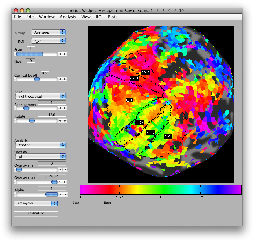
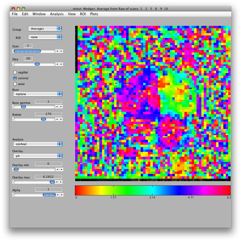
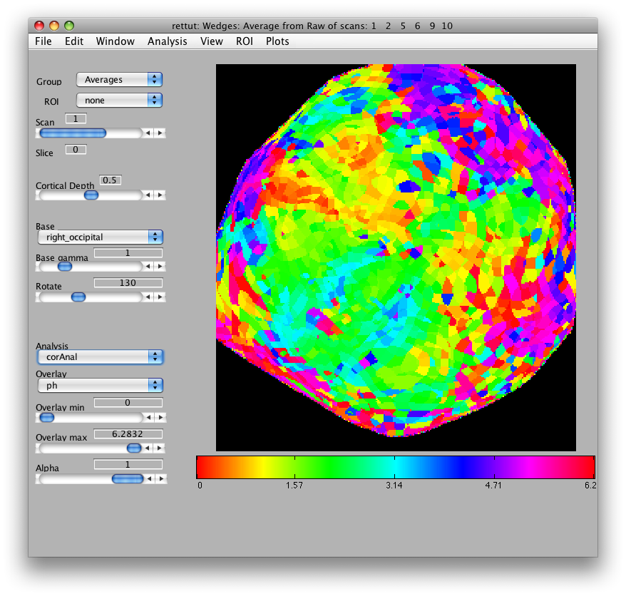
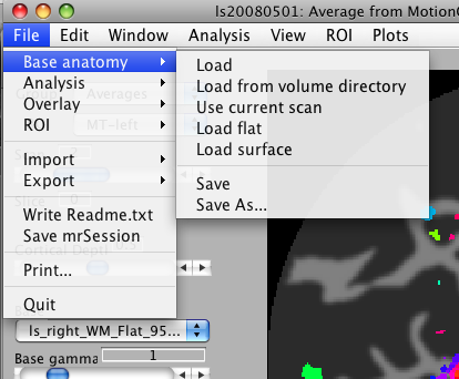
Now, load the flat patch of the right occipital cortex as your base anatomy. Go to File/Base Anatomy/Load and load the file right_occipital.img. If you go back to viewing the ph overlay on Scan 1, you should see:
This is the phase map for the wedges, so the color represents the polar angle of the visual field. We can switch to scan 2 and look at the eccentricity map as well. To do that switch the slider to Scan 2.
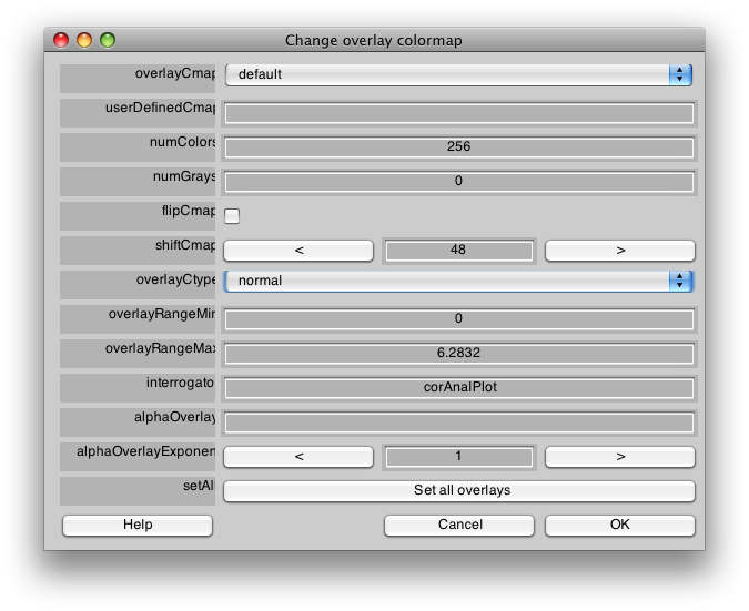
There are a few visualization settings that are also useful to play around with now. One, is to not show voxels that have low coherence with the stimulus. You can do that by choosing the co Overlay in the drop down menu on the main window, and then setting the Overlay min to say 0.3. Now switch back to the ph Overlay and you should see only voxels with high coherence with the stimulus. You can also change the colormap if you like, to do that go to Edit/Overlay/Edit Overlay and you will get a dialog like the following:
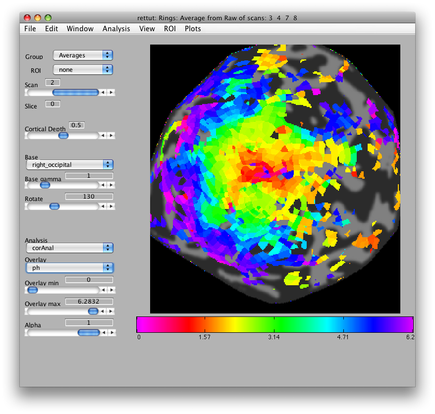
If you shiftCmap by 48, you should get a map that looks like this:
10. Defining visual fields
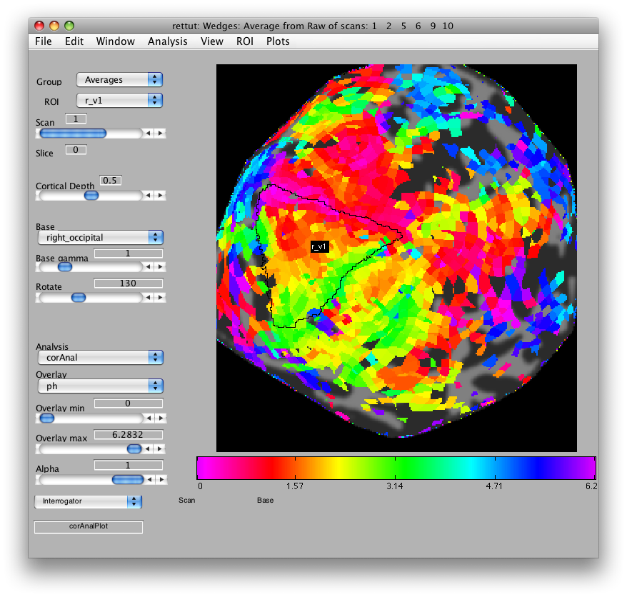
Now, looking at the right_occipital flat map, set the Overlay min to about 0.2 co value and switch back to the ph Overlay. The red/pink points are the lower vertical meridian and the greenish points are the upper vertical meridian. V1 covers the whole contralateral hemifield, so we start by marking off an ROI the spans these two meridians. Go to ROI/Create/Polygon and then give the ROI the name r_v1. Then place points to mark off the area shown below. When you are done marking off the area, double-click:
Note that if you are unhappy with the ROI drawing tool (e.g. it is very slow), you can change how it works in Edit/Preference/roiPolygonMethod.
Now, you can draw r_v2d using the same method, by drawing from the lower vertical meridian to the horizontal meridian (yellowish color) and then r_v3d as the horizontal meridian to the lower vertical meridian. Then, similarly for the ventral parts of v2 and v3, you draw from the upper vertical meridian (green) to the horizontal meridian (yellow) and back again. Finally, we draw (though there is some controversy on this issue) V4 as the full hemifield map below v3v. Of course, there are many other visual areas that you can be able to define. For more information on other areas we routinely define, see Larsson & Heeger (2006) and Schluppeck, Glimcher & Heeger (2005) and references therein. and It should look something like:
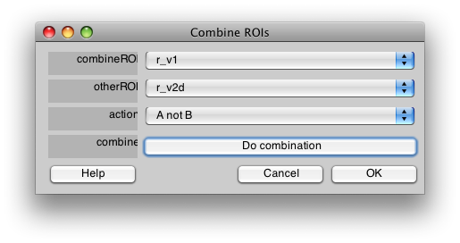
If you want to make sure that ROIs do not overlay each other, you can use the combine tool in ROI/Combine. For instance if you want to make sure that r_v1 has no voxels from r_v2d you would set up the dialog like this:
and press Do combination.
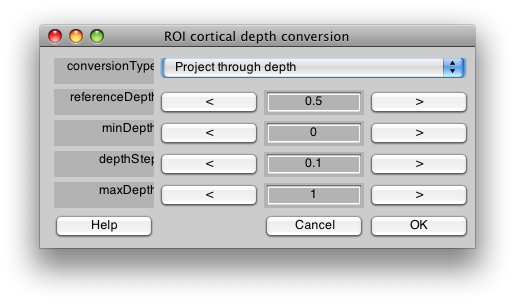
Finally, you may want to extend your ROIs through the cortical depth. Note that by default you are looking at the midcortical depth (See Cortical Depth slider on the main viewer). If you want your ROIs to extend through the gray matter, you can ROI/Convert/Convert cortical depth. You want to Project through depth, and then starting at your current depth (0.5) copy the ROI through the whole gray matter. So you set referenceDepth to 0.5 and then starting at 0 (minDepth) go in increments of 0.1 (depthStep) until reaching the maxDepth of 1, adding voxels that are in the same location to the ROI. Be aware that if you extend too far with your ROI, you may start to cross sulcal boundaries, so use this tool carefully. Also, this tool will only convert voxels if they exist in the currently displayed flat map - so if you want to do rois on the other hemisphere, you will have to switch to the other hemispheres flatmap and convert those rois separately:
When you are done, save your ROIs from the File/ROI/Save all menu item.
Ok! That's it. When you quit through the menu item, you might find that it takes a bit of time to close. This is because mrLoadRet is saving your settings into a file called mrLastView.mat so that when you start again everything will be back in the same place you left it. If you don't want to save your settings, you can always type mrQuit(0) at the command line and mrLoadRet will close without saving. Or, the next time you run, you can run mrLoadRet with mrLoadRet([]) and it will run without loading the mrLastView.mat file. Be aware that until you explicitly save ROIs through the File menu, the ROIs only exist in the mrLastView.mat. Your correlation analysis and the averaging on the other hand has already been saved to disk. You can always reload the Analysis from the File/Analysis/Load menu item.
One last thing that is worth mentioning here. If you don't like all the dialog box warnings, you should set Edit/Preferences/Verbose to “No”. This will print all warnings and errors to the Matlab buffer, so be sure to check there to make sure you don't miss important messages. Also, if the code crashes at some point, it may put you into the Matlab debug mode, that looks like this:
K>>
If you see this happening, you should note what error occurred and then get out of debug mode by typing
K>> dbquit
Note that you can reduce the number of such occurrences by using the GUI in the way that it is intended. A large number of crashes occur because people click on the red button at the top the figure to close it rather than using the Quit/Close menu item or using a button on the GUI like OK/Cancel to close. When you click the red button to close a figure it does not allow the close code to run and the GUI can crash (this is mostly harmless, but can be annoying). You should be especially careful to use the File/Quit menu item from the main GUI to close MLR since that will guarantee that the next time you load the viewer, you will return to the same state of the viewer including all the same loaded Anatomies, ROIs and Analyses.
-jg.
Event Related Tutorial
This tutorial will show you how to run an event-related analysis. Note that the Retinotopy Tutorial is the best place to start for a full introduction to using mrLoadRet. This tutorial starts after the initial steps of running mrInit, the Motion Compensation and Alignment – those steps are described in the retinotopy tutorial. The experiment that is being analyzed here is one in which the subject viewed randomly moving dots. On each trial, the dots moved coherently for a couple of seconds in one of three directions, and then went back to moving incoherently for several seconds. Thus there are three different trial types that will be deconvolved, for each of the three directions of motion, and we will look at the responses in MT.
Overview
- Download the tutorial files
- Concatenate scans together
- Set stimfiles
- Run event-related analysis
- Viewing the analysis
1. Download
You can download the tutorial files from:
Note that this is a rather large file. Approximately 300MB.
The files are provided as a tar/zip file. In Mac OS X you should be able to just click to open the files in the Finder. Otherwise, you can go to a terminal and do:
gunzip erTutorial.tar.gz
tar xvf erTutorial.tar
We assume that you have mrTools running on your system.
2. Concatenate
Start up Matlab and switch to the erTutorial directory you just downloaded, and run mrLoadRet:
cd erTutorial
mrLoadRet
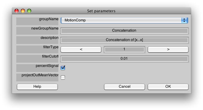
We are going to run a concatenation. The purpose of concatenating scans together is first to make a single long scan out of a few shorter scans so that we can estimate the responses using all the data. Second, this step runs preprocessing steps on the data such as high-pass filtering and converting to percent signal change.
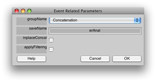
Make sure the Group tab is set to MotionComp and then Select Concatenate Time Series from the Analysis menu. You should see a dialog like the following:
We do not need to change anything on this dialog to have it run. For a description of the meaning of the parameters press help, or see the Event Related manual pages.
Press OK.
You will see another dialog where you should select all the scans for concatenating:
Press OK. This will take a few minutes to run.
3. Set stimfiles
We will now tell mrLoadRet which “stimfiles” to use for these scans. Stimfiles contain the information about the timing of events in the experiment that is used for the deconvolution analysis. Note that we set the stimfiles on the Raw TSeries (i.e. the original time series). This can be done before or after the concatenation is done. The concatenation scan has saved what original scans and from what group it came from. So, to find the correct stimfiles, mrLoadRet always checks back to those scans to see what stimfiles they are linked to. This way, you can always change how you have linked the stimfiles at any given time.
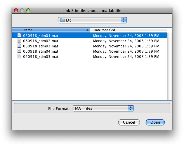
Switch the Group tab to Raw. Go to Scan 1. Now go to the Edit menu and select Edit/Scan/Link Stimfile. You should get a file choosing dialog like this:
Choose to link the first scan with the first stimfile “stimvol01.mat” and click Open.
Now, Set the scan slider to 2, and repeat this process, linking scan 2 with stimvol02.mat.
Link all the rest of the scans accordingly, (i.e. Scan 3 → stimvol03, Scan 4 → stimvol04 and Scan 5 → stimvol05).
While this is a bit tedious, the process can be automated for a real experiment you run, and the mrInit dialog makes it easier to link all the stimfiles at one time when you first start your session.
Now, let's go check to make sure that you have linked the files correctly.
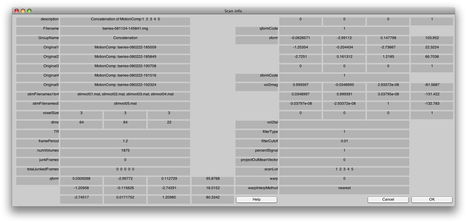
Switch to the Concatenation Group, and then choose the Edit/Scan/Info menu item.
You should see something like the following:
In particular, check that the stimFilenames are listed in sequential order. If they are not, switch back to the Raw group and fix it by re-linking the stimfiles again.
The stimfile format used here is very simple. It is a cell array where each element in the cell array is for a different trial type (in this case different directions of dot motion). Each element of the cell array consists of an array whose elements list the volume number that the stimulus occurred on. There is also a stimNames cell array that gives what the names of the trial types are. You can see what this looks like, by doing (from the matlab command line);
v = newView;
stimfile = viewGet(v,'stimfile',1,1);
and you should see that it looks like:
  >> stimfile{1}

ans =

      stimvol: {[21 38 60 75 96 104 150 156 181 195 223 256 285 300 305 332 364]  [1x18 double]  [1x17 double]}
    stimNames: {'Direction: 35 deg'  'Direction: 135 deg'  'Direction: 255 deg'}
     filetype: 'stimvol'
For a description on how to create your own stimfiles see the Event Related manual pages.
4. Event Related Analysis
Now, let's run the event-related analysis. Select Event-related analysis from the Analysis menu, and you should see the following dialog:
You should select “applyFiltering”. This checkbox filters the columns of the event-related design matrix in the same way that the data have been filtered (i.e. high-pass filtering). Click OK.
Select the single scan in the next dialog box, and click OK.
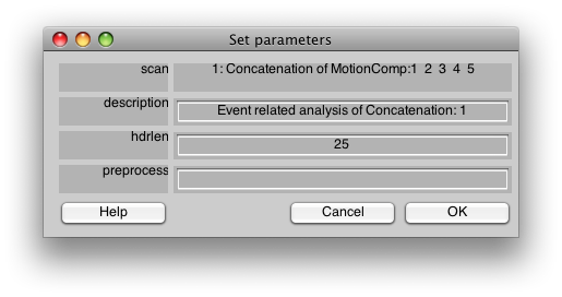
You should now see:
This is the dialog which chooses some information about how to do the event-related analysis. The hdrlen is the length of the response to calculate in the deconvolution.
Click OK.
Running the analysis will take a few minutes. Note that if you are on a system that does not have very much memory, you can choose to have mrLoadRet break up the computation into smaller chunks. This is set in the Edit/Preferences dialog. The smaller the chunks the longer it will take to calculate, but use less memory.
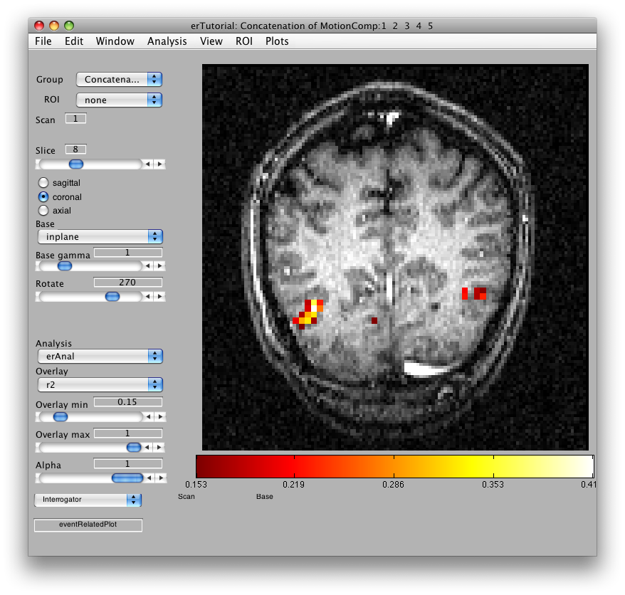
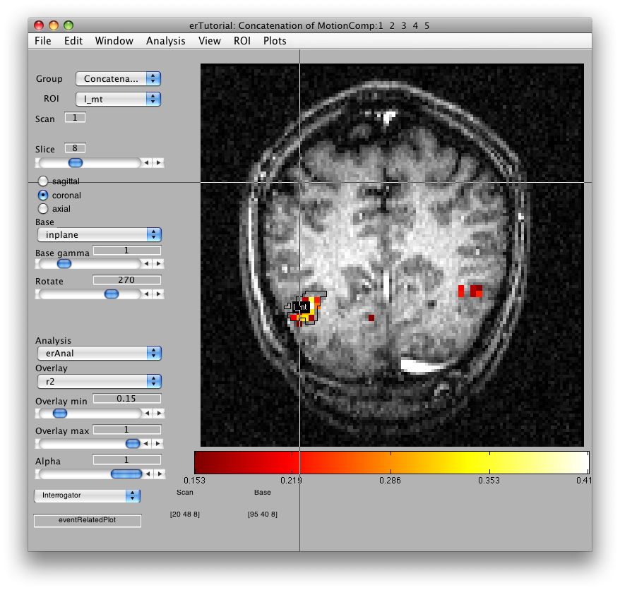
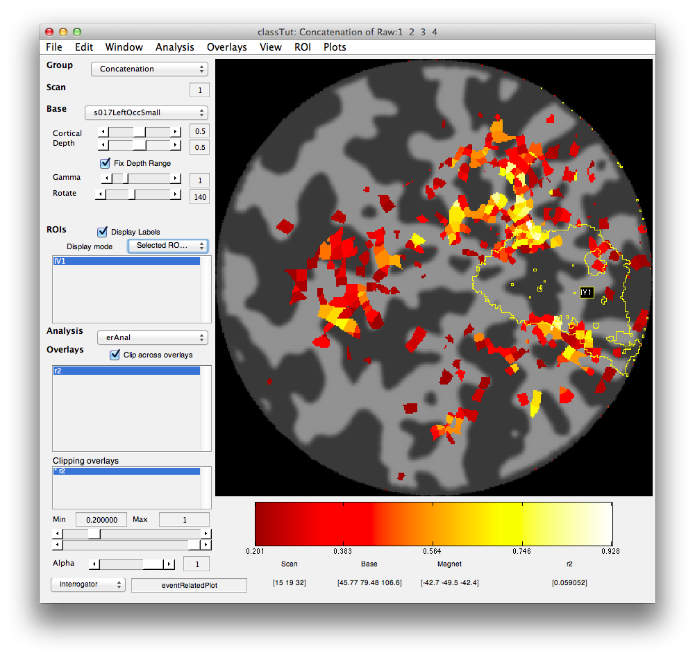
Once the analysis is complete, set the overlay min to 0.2 and the Slice slider to 8, and you should something like the following:
This is an r2 map of the event-related analysis. It tells you what proportion of the variance in each timecourse is accounted for by the average hemodynamic response See Gardner et al., Neuron (2005) 47:607-20, for more information.
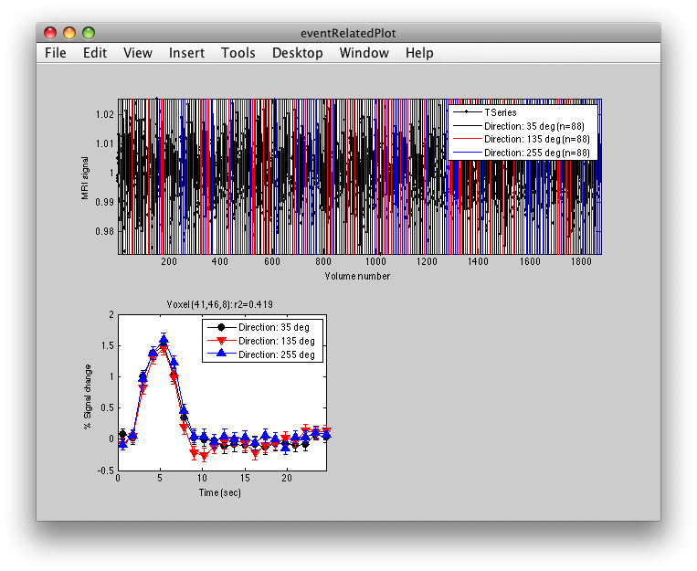
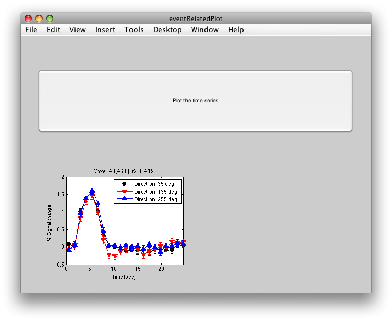
To see what the responses look like at any individual voxel, turn on the interrogator (Plots/Interrogate Overlay) and you should see “eventRelatedPlot” in the text box in the bottom left (see above figure). Go ahead and move the cross-hairs over the voxel with the highest r2 value (white) and click. You should then see:
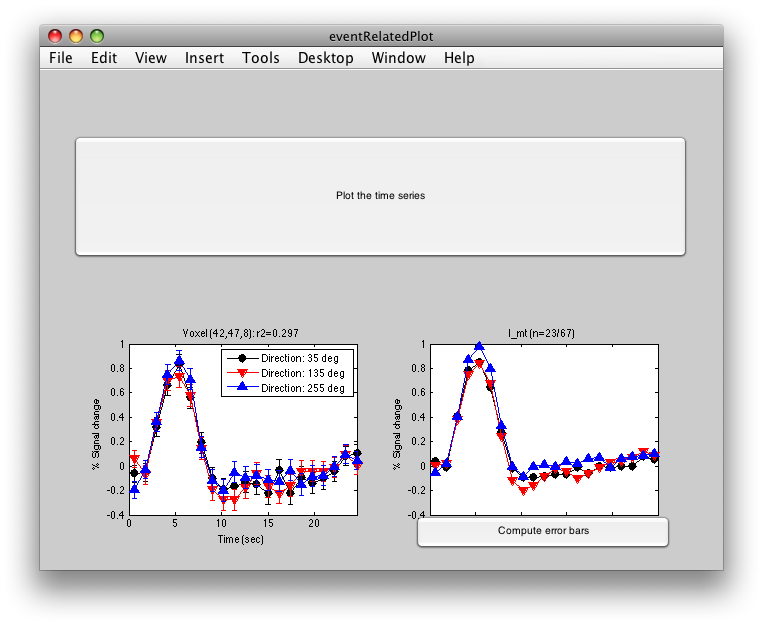
This shows the three deconvolved responses to the three different trial types. If you click on the button to Plot the time series, you will see:
This shows the time series at the top, with a vertical line every time one of the trials occurred. Note that the time course is in percent signal change, and has been set to have a mean of 1. This is what the concatenation code does. The mean is set to 1, so that if you divide by the mean again (to get percent signal change), nothing will change in the time series.
You can also look at average responses across an ROI. To do that, load the l_mt roi, by using File/ROI/Load. You should now see:
Click inside the l_mt roi and you will get:
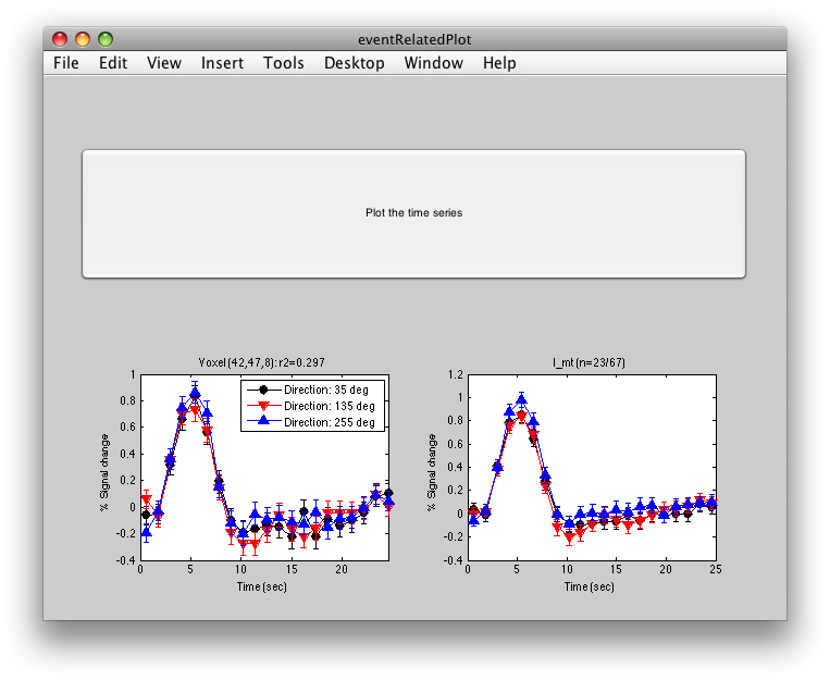
The graph on the left shows the individual voxel you clicked on. The graph on the right shows the deconvolution averaged across all the voxels in the l_mt ROI that meet the r2 cutoff that you set in the Overlay Min. This display simply averages across the already computed deconvolved responses. If you want to get error bars, click the “Compute Error bars” button, and after a little bit, you should see:
What this does, is reloads all the time courses that meet the r2 cutoff set by the overlay min and then averages those time courses together into a single time course. It then recomputes the deconvolution analysis on this average time course. The error bars are now standard errors over the number of repeats of the stimulus. (Technically, they are computed as the residual variance distributed back to each time point in the deconvolved response according to the inverse of the covariance of the design matrix).
-jg.
Surfaces and Flat Maps Tutorial
This tutorial will show you how to import a surface segmentation into mrLoadRet so that you can view your data on a surface. It will also show you how to make a flat map from that surface.
Overview
- Download tutorial data
- Create a curvature file
- Load event-related analysis to view on inplane anatomy
- Import surface
- Create a flatmap
- Finding voxels in different anatomies
- Inflated surface
1. Download
You can download the tutorial files from:
The files are provided as a tar/zip file. In Mac OS X you should be able to just click to open the files in the Finder. Otherwise, you can go to a terminal and do:
gunzip surfTutorial.tar.gz
tar xvf surfTutorial.tar
We assume that you have mrTools running on your system. This is a paired down version of the same dataset as the Event-related Tutorial. To make it easier to download it does not include all the data files, so you cannot rerun analyses on this example. The data has already been motion corrected, aligned to the 3D volume using mrAlign, concatenated and the eventRelated analysis has been run.
2. Create curvature
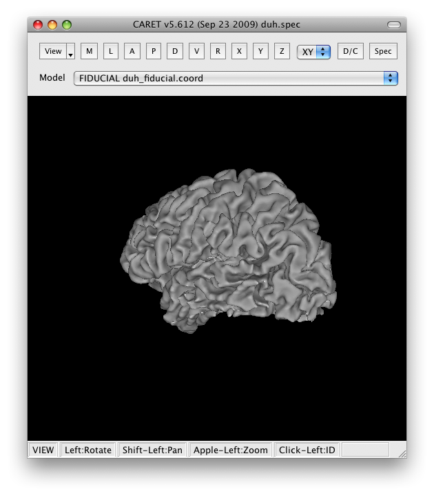
To view your data on a surface, mrLoadRet needs a segmentation. A segmentation consists of two surfaces, one that tells where the outer (pial) layer of the gray matter is and one that tells where the inner layer is (between the white matter and the gray matter). These files can be created by any segmentation tool as long as they are in .off format. We typically use FreeSurfer (see here for how to import) to generate segmentations. Jonas Larsson's SurfRelax and Caret (though Caret only produces a mid-cortex surface and not the outer and inner surface as we like to use. see here to import) can also be used.
Once you have a segmentation, mrLoadRet also needs a file which tells it how to color the surface. We use the curvature to color the surface. In this tutorial we have provided an outer and inner surface for the left cortex, but no curvature file. You thus need to create the curvature file:
First cd into the Segmentation folder:
cd Segmentation
You should see the following files:
>> ls
leftOuter.off     volume.img
leftInner.off     volume.hdr
Now generate the curvature from the inner surface
m = calcCurvature('leftInner','leftOuter');
And then save it in vff format:
saveVFF('leftCurvature.vff',m)
3. Display event-related Analysis
First, we will start up mrLoadRet
cd surfTutorial
mrLoadRet
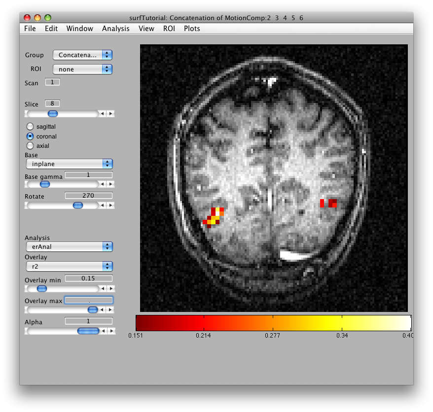
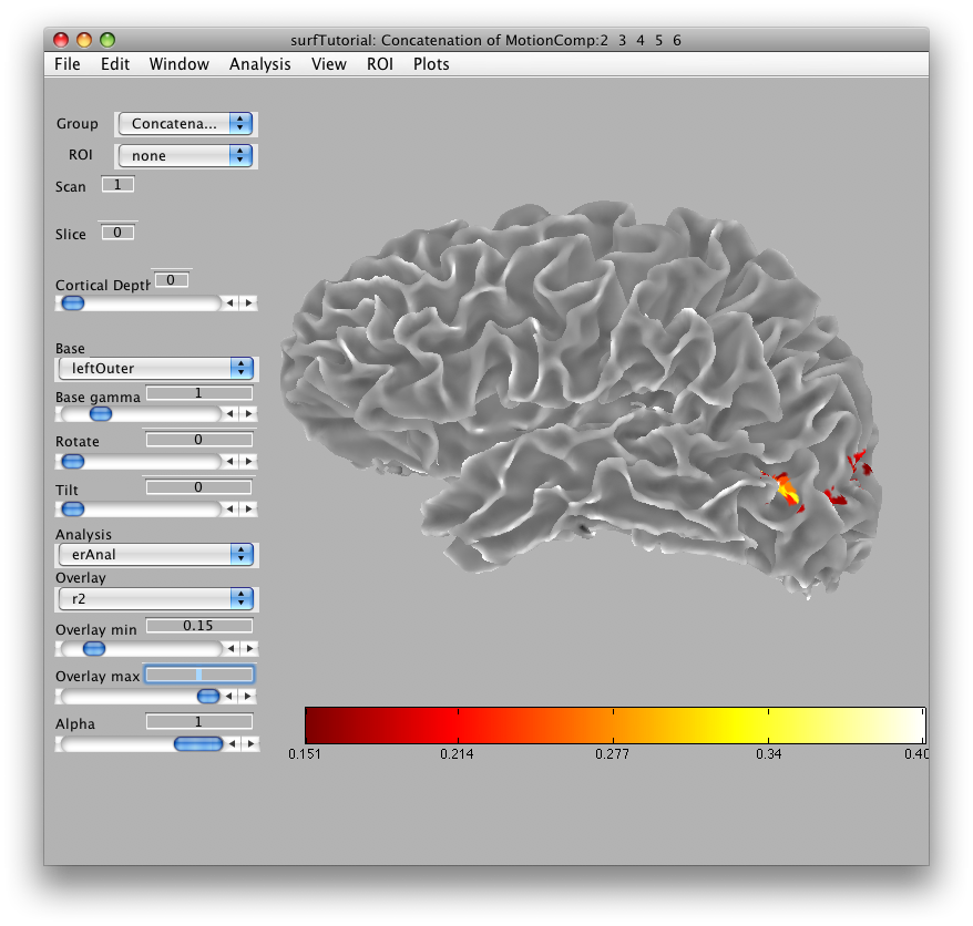
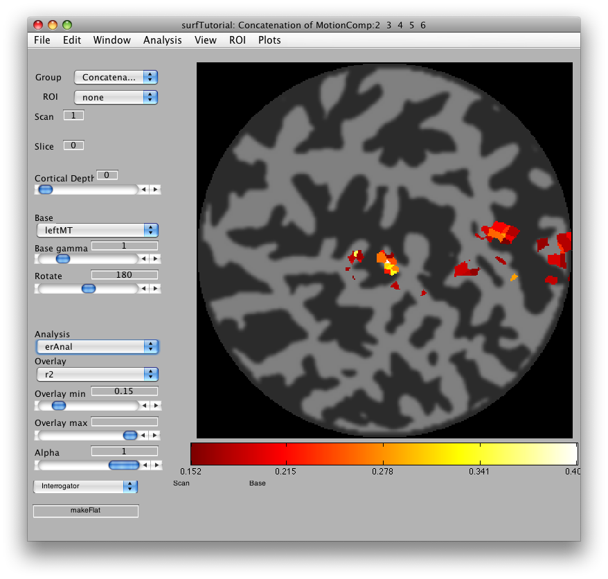
Then we will load the already computed event-related analysis and view it on the 2D inplane anatomy. Make sure you are on the Concatenation group and then from File/Analysis/Load, load erAnal/erAnal.mat. Set the Overlay Min to 0.15, the Slice to 8, and you should see (you might need to go to slice 15 and set Rotate to 90):
4. Import surface
Now, we are ready to import the surface. Go to File/Base Anatomy/Import Surface, and find the outer surface file in the segmentation directory (i.e. Segmentation/leftOuter.off) and click Open.
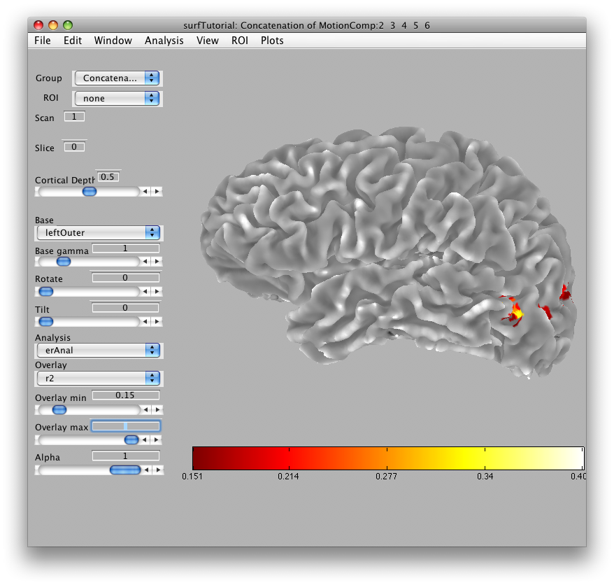
You should now see a view of the surface like this:
With a set of controls that look like:
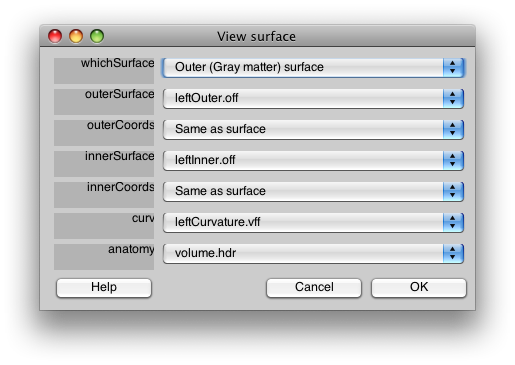
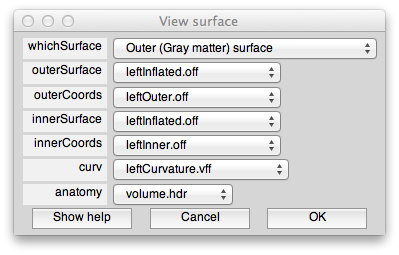
This dialog should have the correct settings to load your surface already, but it allows you to make changes and selections. The surfaces appear four times in the dialog. This is because there is a distinction between a display surface and a coords surface. The display surface is the surface that will be actually drawn. The coords surface specifies where the data for the displayed surface comes from. In our case these are one and the same, but if you were displaying on an inflated surface, for example, you would want the display surface to be the inflated surface and the coords surface to be the gray matter surface. The outer and inner surfaces are what will be displayed when the cortical depth slider (more later on this) is set to 1 and 0, respectively.
The other files you see here are the curvature file which is simply how to color the surface. The anatomy file is the 3D volume anatomy from which these surfaces were segmented. It is important to have this file since it contains the right transformation matrix that is needed to transform data on to the surface to be displayed.
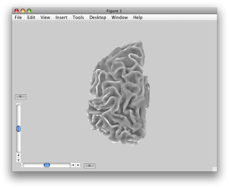
At the top of the dialog, you will see a field called “whichSurface” this chooses which surface that is currently being displayed. This is there so that you can inspect all the surfaces to make sure you have chosen the right one. For example, set it to Inner (White matter) surface, and you should see:
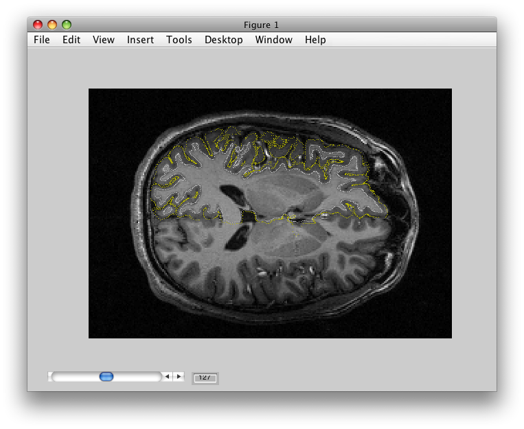
If you set whichSurface to 3D Anatomy, you should see this:
The 3D Anatomy is particularly important to inspect. The yellow line shows you where the outer coords are being taken from. It should follow the outer surface of the gray matter. The data that will be displayed will always come from the location of where the yellow line is, if you set the cortical depth to 1. There is also a white line. This should follow the inner surface of the gray matter. It is where data will be interpolated from when you set the cortical depth to 0. When you set the cortical depth to an intermediate value (e.g. 0.7) it will interpolate the data from the appropriate depth between the inner and outer surface.
Again, it is a very good idea to look at this view carefully to understand how good your segmentation was.
When you are done, click OK.
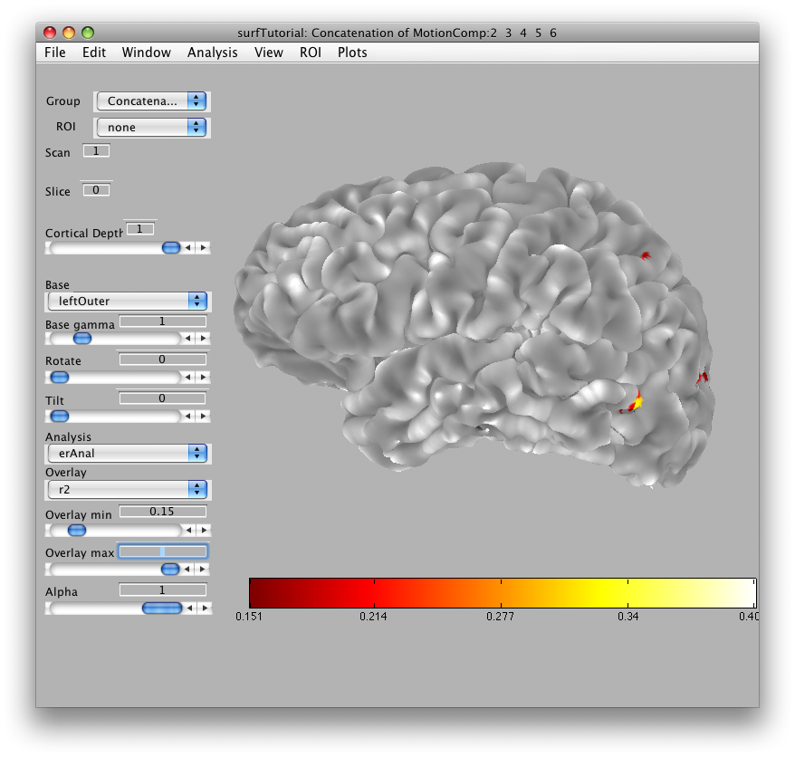
In a moment, you should see in the main viewer, something like this:
You can use the rotate and tilt sliders to rotate and tilt the surface. You can also change the cortical depth that is being displayed. When you set the cortical depth to 1, you will see the outer surface:
When you set the cortical depth to 0, you should see the inner surface:
Note that if you ever want to go back to look at the files that created the surface, you can always go to Plots/Surface Viewer.
Now that you have imported the surface, you may want to save it in a format the MLR can read directly. First, you may want to change its name, which you can do by going to Edit/Base Anatomy/Edit Base Anatomy and then setting the baseAnatomy. Next, go and save by going to File/Base Anatomy/Save. This will save a file that can be directly read back into MLR without importing into the Anatomy directory. If you wanted to save to a different directory (for instance the volumeDirectory repository which you should set in Edit/Preferences volumeDirectory), then click on File/Base Anatomy/Save As… and it will bring up file save dialog which opens up to the Edit/Preferences volumeDirectory.
5. Make a flat patch
Now that you have the surface loaded, it is easy to make a flat patch of any location you want.
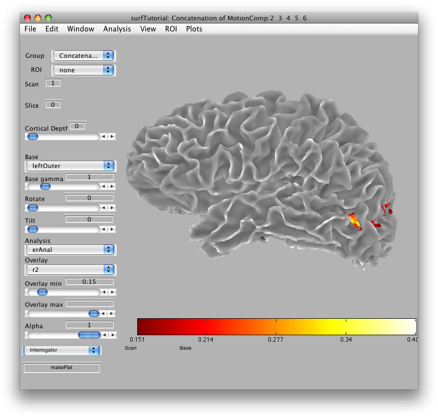
Go to Plots/Interrogator Overlay and turn the interrogator on (by clicking). In the bottom left of the viewer, select “makeFlat” as the interrogator from the drop down list box, so that makeFlat should now appear in the text box at the bottom left of the viewer:
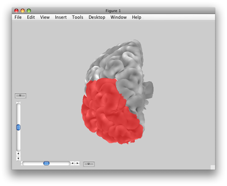
You can now click on any portion of the surface that you want to flatten. For instance, the patch of brightly colored voxels that you see in the mid-occipital cortex is MT. Click on that, and you should see a preview of the flat patch to be made that looks like:
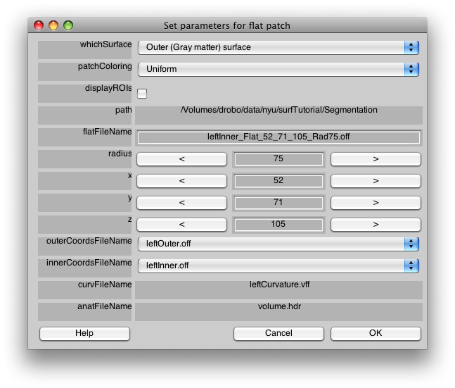
And you will get a parameter dialog that looks like:
Like last time, you can look at the various surfaces, by changing “whichSurface”. You can also change the way the patch is colored, for example, try “Current Overlay with Patch” in “patchColoring” and then you should be able to tell if the patch you are making covers the whole area of activated cortex that you are interested in. You can also change the radius of the patch to make it bigger or smaller.
The only parameter we need to change though is the name. Change the flatFileName “leftInner_Flat_52_71_105_Rad75.off” to “leftMT” and click OK>
You should then see the following dialog:
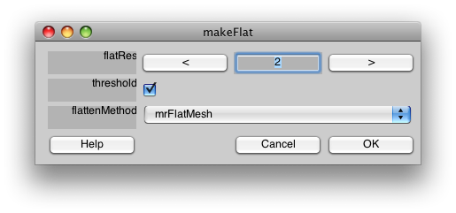
The flatRes is the “resolution” of the flat patch. The flat patch will be converted from a true surface into a 2D image, and the resolution refers to how high a resolution you want to represent that flat image with. 2 is usually a good number, but if the resulting flat patch looks pixellated, you may try a higher resolution. The threshold check box, will make it so that the curvature is threshold, making a two color flat patch. If you want to have the smooth curvature displayed instead, turn off the threshold.
flattenMethod selects which system to use to flatten the patch. We typically use mrFlatMesh, which is a modified version of the code that came from the Stanford Vista package developed by Brian Wandell's lab. If you are using Jonas Larsson's SurfRelax tools and have those properly installed, you can choose SurfRelax and try that.
Select mrFlatMesh as the flattenMethod and click OK. After a few minutes, you should see:
Note that you may need to rotate the patch to get it in the same orientation. In general, you should try to orient your patches such that dorsal is up and ventral is down - the next section which shows you how to search for voxels is useful for this, particular in the “continuous mode” described below which will show you which part of the patch is at the top and bottom of the brain.
You are now done making your first flat patch.
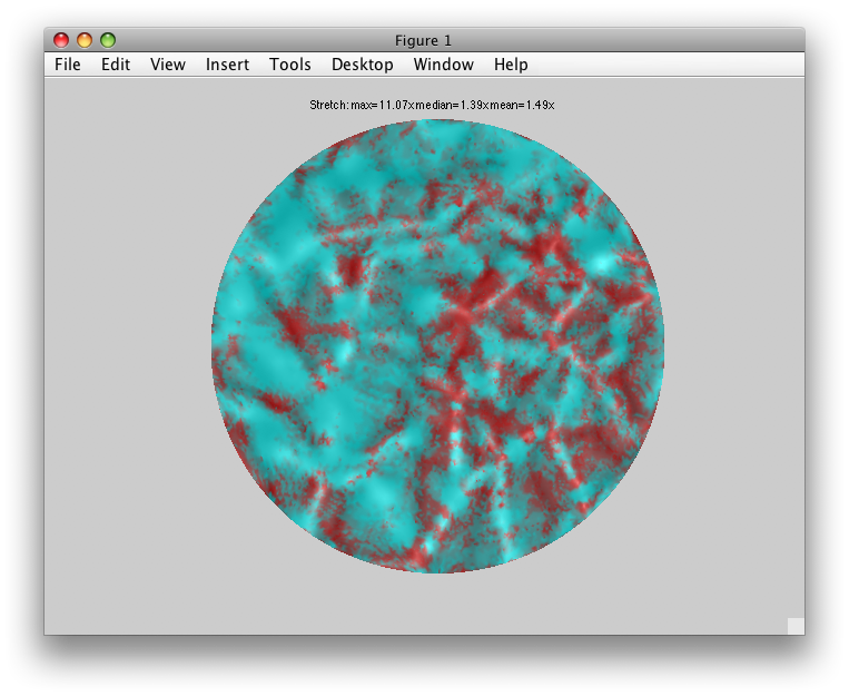
If you want to go back to the view of the flat patch on the surface, you can select Plots/Flat Viewer. This is a useful thing to do, since you can also see how the patch is oriented and see how much distortion is in the patch.
For example, from the Flat Viewer, select “whichSurface” to be “Patch” and “patchColoring” to be “Stretched areas in Red”. You should see something like:
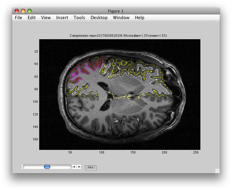
You may also want to see where your patch coordinates are coming from on the volume anatomy. Choose “patchColoring” to be “Uniform” and “whichSurface” to be “3D Anatomy” and you should see:
The yellow and white are the same as before (your outer and inner surface boundaries). But, the Red and Pink parts are the outer and inner coords for your flat patch.
You can click OK to get out of the Flat Viewer.
You may also now want to change the baseName and save the flat patch to a native MLR format (nifti pair with associated matlab file) by following the directions above at the end of the section on Importing a surface. Note that when you save it will save the default rotation and other parameters so that the next time you load it the flat patch will be oriented correctly.
6. Finding a voxel
Some times it can be very confusing looking at a flat patch and deciding where a particular voxel of data came from. One way to figure that out is to use the “searchForVoxel” interrogator.
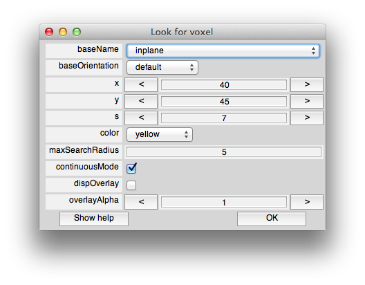
You should still have the interrogator on (Plots/Interrogator). Now select searchForVoxel in the drop down list box at the bottom left of the viewer, and “searchForVoxel” should now appear in the iterrogator text box. Now if you click on one of the activated voxels in the center of the patch, you should get a dialog like this:
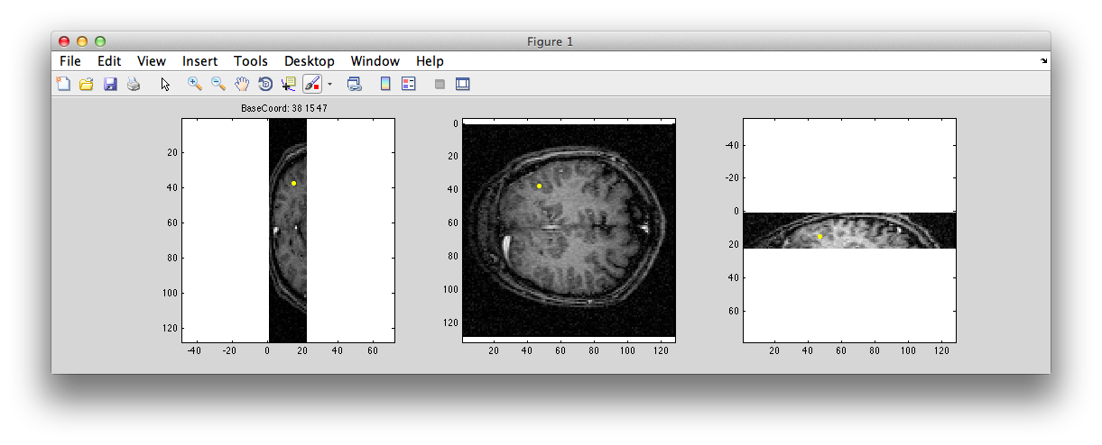
Assuming continuousMode is checked, then as you move your mouse over the flat patch in the main viewer, you should see a little yellow dot move around in another figure window that pops up like this:
The little yellow dot should run around in there as you move the mouse over the flat in the main viewer indicating its location in the inplane anatomy. This can be very helpful in determining where points came from in the flat. If you have a full 3D canonical available (not in this tutorial), you could switch to that anatomy in the dialog box shown above and it will show you in that anatomy.
The following feature has been a bit superseded by the continuous mode (you can avoid doing it by closing the dialog box by clicking on the red x button at the top left), but if you choose “inplane” for the baseName, and set the color to purple (so that it will be easier to see) and click OK, then it should switch you in the main viewer to the inplane anatomy and it should look like this:
Notice the four purple little points that are drawn over one of the voxels on the left side. This is where the voxel you clicked on in the surface came from.
7. Inflated surface
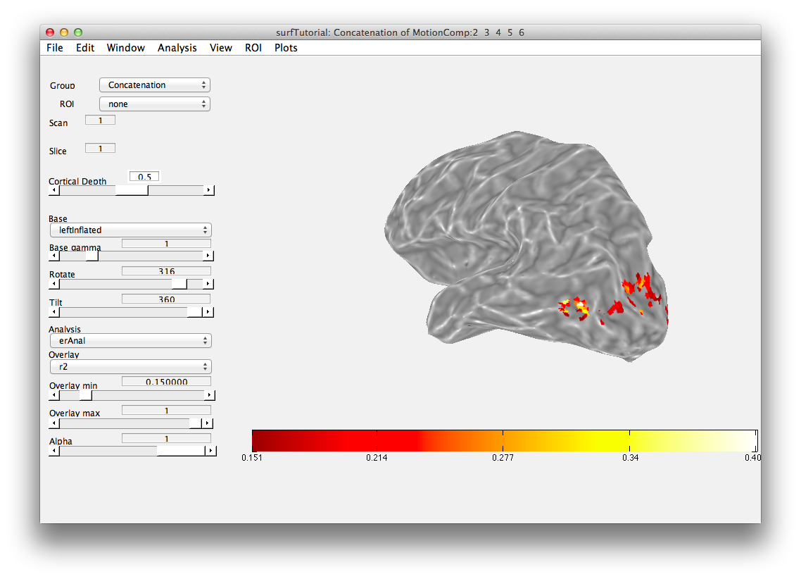
Often it is convenient to make an inflated surface to display your data on. This is easy to do by using the inflated surface that FreeSurfer creates. Go to File/Base Anatomy/Import Surface, find leftInflated.off from the Segmentation directory. Now you just have to set the outer and inner coords appropriately (obviously you don't want to use the coordinates of the inflated surface since those are in the wrong place and should be used for visualization only). Your dialog should look like this:
When you click ok, you should get a surface in the viewer that looks like this:
-jg.
pRF Tutorial
This tutorial shows you how to run a pRF analysis (see Dumoulin and Wandell (2008) for details - also Kay, Naselaris, Prenger and Gallant (2008)) with mrTools. The basic idea of a pRF analysis is to fit a “population receptive field” to each voxel. This is usually based on stimuli similar to a typical retinotopy experiment (rotating wedges, rings and moving bars). The responses to these stimuli are predicted by a very simple gaussian receptive field model. The gaussian RF has parameters of x,y position and standard deviation (receptive field size). Then for any give gaussian RF one can generate a model time series by simply multiplying the gaussian by the stimulus time-point by time-point and taking the sum across space. This gives a time series (i.e. the response of the receptive field to the stimulus). Convolving this with a standard hemodynamic function (or in some cases a parameterized one with fit parameters that one can adjust) produces a model time series. Then one finds the RF parameters that produces a model time series that most closely matches the actually measured time series for a voxel. This then is taken as the best population RF for that voxel. By doing this you can get the usual information that you get from a retinotopy experiment (the eccentricity and polar angle for the RF of each voxel), but also as a bonus the receptive field size as well. Plus you are not restricted to stimuli that produce a response that is sinusoidally modulated in time (like wedges and rings). You can in principle use any stimulus that causes response modulation (like bars or white noise).
You should have already run the retinotopy tutorial before going through this tutorial.
Overview
- Download the tutorial files
- The stimuli used in the experiment
- Do the classic retinotopy as a reference
- Average and concatenate appropriate scans
- Run pRF analysis on V1 bars
- Examining output of pRF analysis
- Constrained search
- Prefit
- Fitting hemodynamic response function
- Running a full analysis on V1
1. Download files
You can download the tutorial files from:
Note that this is a rather big file, approximately 300MB.
The files are provided as a tar/zip file. In Mac OS X you should be able to just click to open the files in the Finder. Otherwise, you can go to a terminal and do:
gunzip pRFTutorial.tar.gz
tar xvf pRFTutorial.tar
We provide you with a set of 10 functional scans, an inplane anatomy file, a flat map of the left occipital cortex and an inflated left occipital surface.
The functional scans include 4 rotating wedge runs (2 CW and 2 CCW rotations) and 2 expanding and contracting ring runs (1 expanding and 1 contracting). Each run is 168 volumes long (a volume was acquired every 1.54 seconds). The first 8 volumes will be thrown out to allow hemodynamic response and longitudinal magnetization to reach steady state for the correlation analysis, but for the pRF analysis all volumes may be kept. The data has already been motion compensated (since this step takes quite a bit of time to run).
From here, all the directions will be for commands to run under Matlab. It is assumed that you have properly set up mrTools using the directions under Getting Started.
Note that if you want to run this on your own subjects, you will need to run the stimulus program mglRetinotopy.
2. Stimuli and analysis
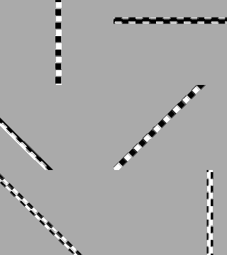
The visual stimuli are the familiar ones from retinotopy which are CW and CCW rotating 90 degree wedges and expanding and contracting rings. But, typically we also run bars stimuli in which a bar sweeps across the visual field in 8 different directions (its important that they sweep both forwards and backwards so that receptive field size and hemodynamic response width are not confounded. Also, we typically run the bars in a pseudo-random order but keep the same order fixed across repeated scans and average all of the data together). Another important point is that it is useful to turn off the stimulus (go to gray) for a cycle every now and then. This probes for very large receptive fields which may not be modulated by stimuli that move within the receptive field. The bars stimuli look something like this (note that the subject typically is fixating in the center on a fixation cross - not depicted - while doing a straight-forward fixation task):
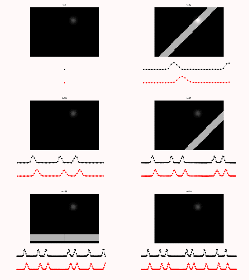
The pRF analysis is basically very simple. We hypothesize that each voxel has a gaussian shaped receptive field (the combined receptive field of the population of neurons which contribute to the response of the voxel). We then want to fit the parameters of this gaussian (x, y and standard deviation) such that the predicted response of the receptive field to the stimuli we presented best matches the actual measured time series. We make predicted responses, like the following:
What you see in the above is a small receptive field in the top right with the stimulus running over it in different directions. The black trace below is the time-point by time-point multiplication of the stimulus and the receptive field summed over all of space (it is the predicted response of the receptive field). That gets convolved with a hemodynamic response function to make the predicted BOLD response in red.
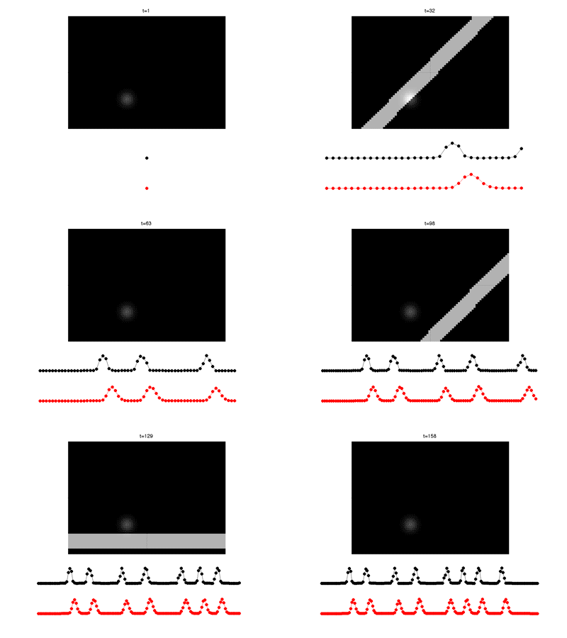
If you move the receptive field to a different location, it predicts a different time series:
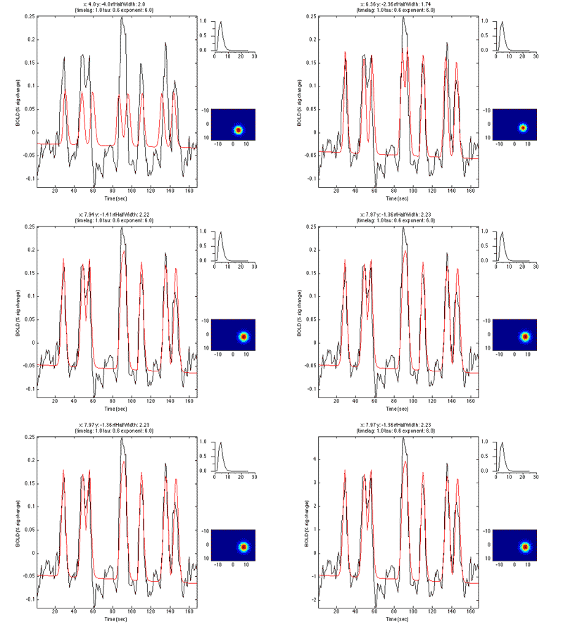
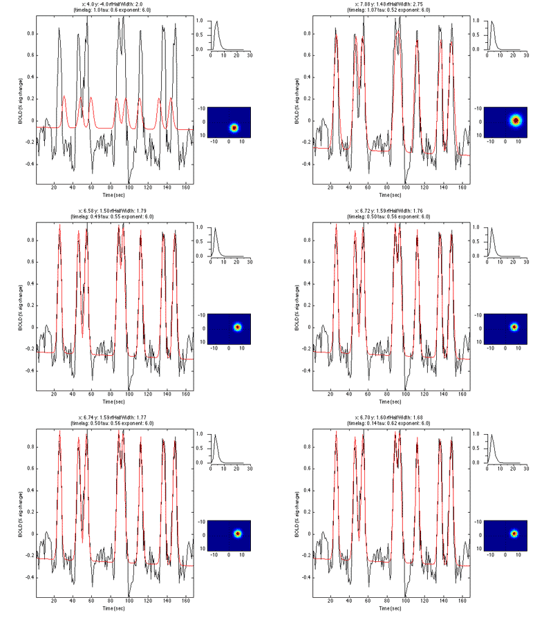
So, to fit a voxels response we change the position and standard deviation of the receptive field until the predicted response (red) best matches (in a least-squares sense) the actual time series for the voxel (note the lag in the BOLD response compared to the black trace).
Here is an example of a fit as it proceeds to change the receptive field position and size to best match the predicted time series (red) to the measured time series for the voxel (black):
3. Retinotopy analysis
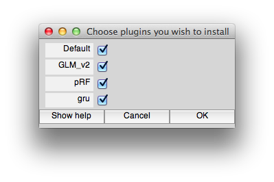
We start by doing a quick retinotopy analysis. This will be used as a reference. We will be using the pRF and GLM_v2 plugins (GLM_V2 provides some better user interface items). Make sure these are installed by doing:
>> mlrPlugin
and selecting from the dialog GLM_V2 and pRF. Note that if you have a mrLoadRet going already, you will need to restart it to have these settings take effect.
Now, go ahead and start mrTools by cd'ing into the experiment directory and running:
>> mrLoadRet
The scans are all labelled and you should be able to do this analysis w/out looking at the cheat sheet below. Note that the best shift used for these scans was -2. So, go ahead and average together appropriate scans with the correct shift and flip and then run the correlation analysis!
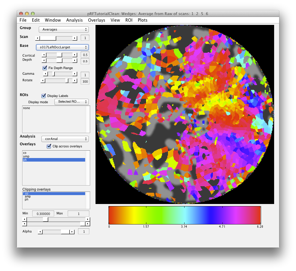
If all went well, your retinotopy should look something like this:
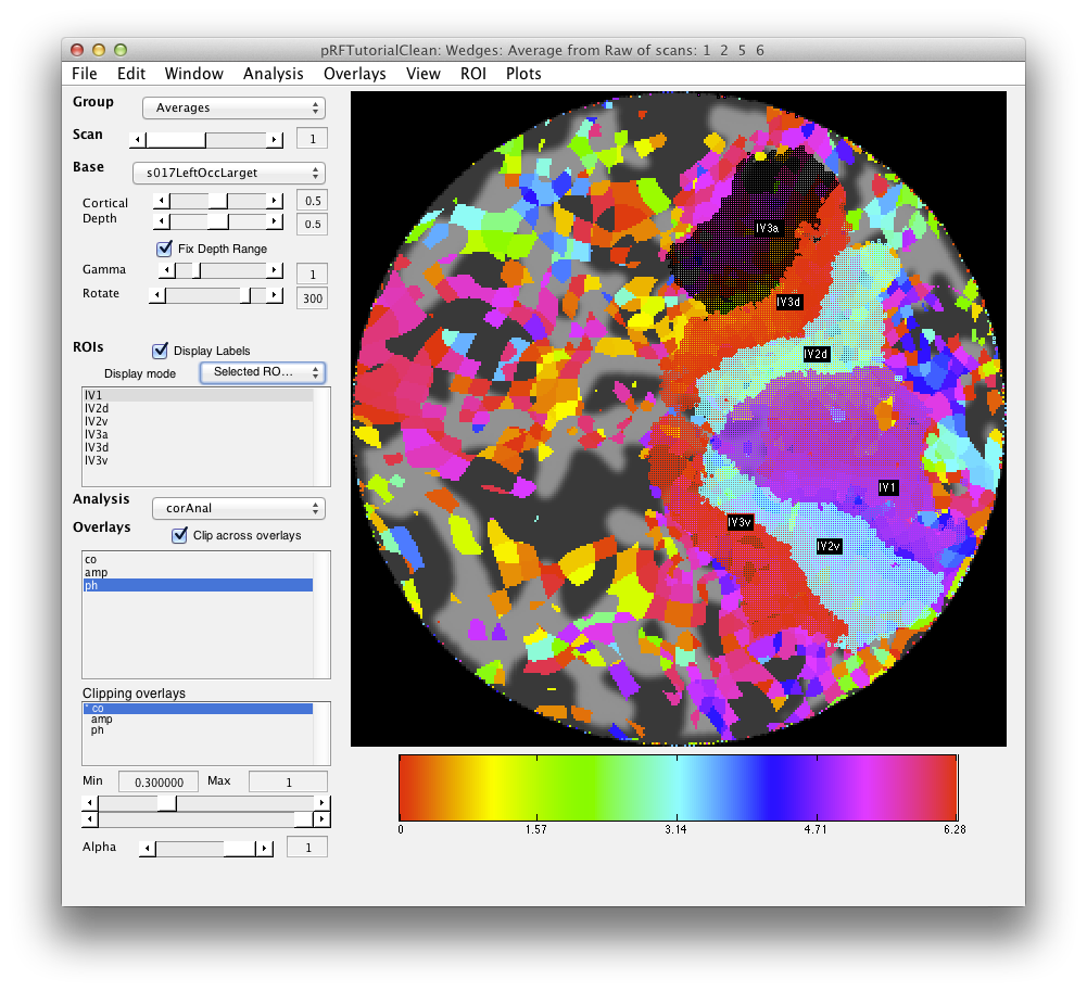
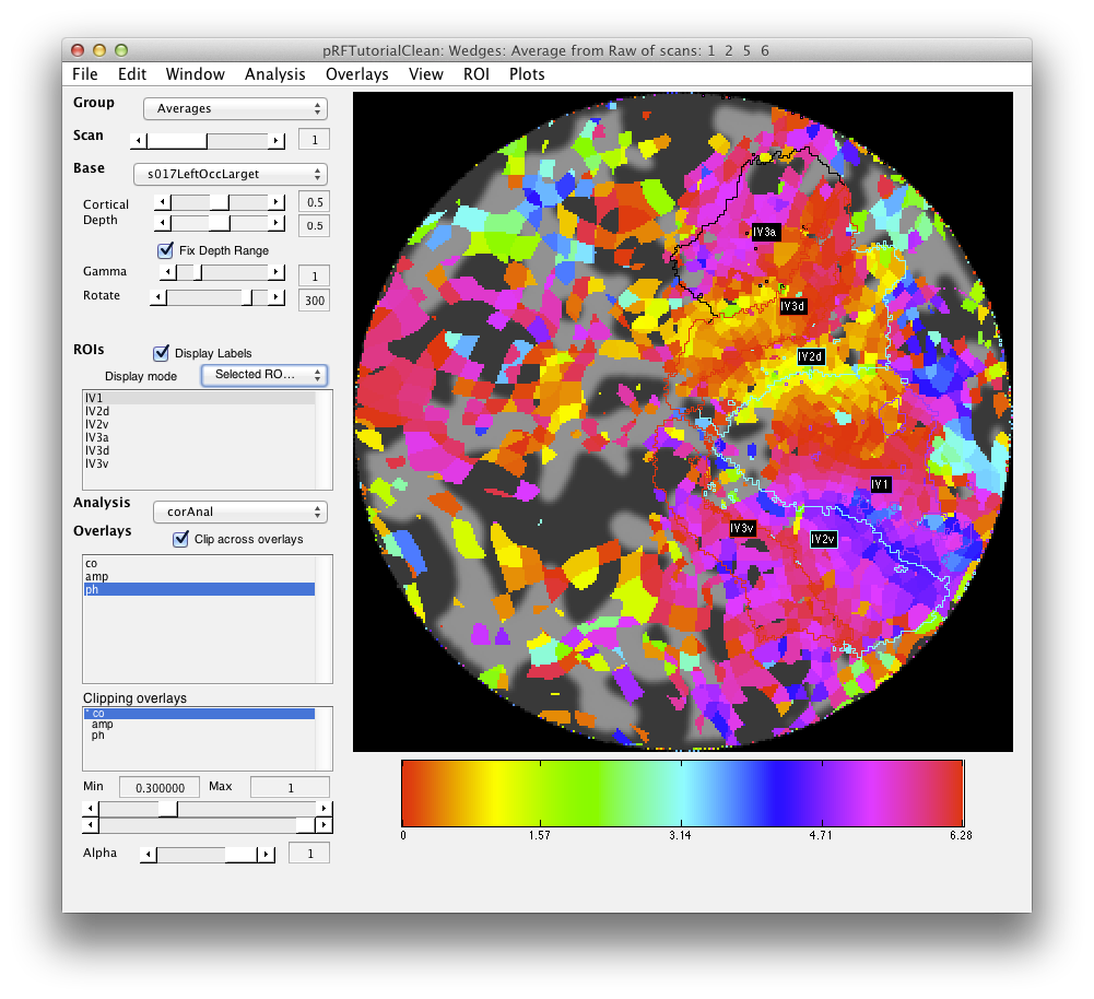
Now you should draw ROIs for V1, V2, V3 and V3a (hV4 is a bit broken up in this particular scan). Again you should be able to do this based on what you learned in the Retinotopy tutorial. For our version check the following:
4. Average and concatenate
In the next steps you will average and concatenate scans for the pRF analysis. Note that this is different from what you do with the retinotopy analysis in which you shift and flip and do other tricks to account for the hemodynamic lag. For pRF analysis you are going to fit a model of the response which has the hemodynamic response lag as part of it. So you don't want to adjust the timing of the scans at all. This is important. If your scan timing is not correct relative to the stimulus all bets are off. In particular, you do not want to shift or reverse scans in averages. The code does handle junkFrames appropriately, but we are going to turn those off too. Remember that if you remove frames then your model has to know you did this otherwise it will associate the wrong stimulus with the response. So, here goes, let's make averages of like scans without any messing with the scans.
- Turn off junk frames in the Raw group: You do this by going to the Raw group (Select from the group dropdown on the top left) and selecting Edit/Group/Edit Group and then go through and set Junk frames to 0 for each scan. This should automatically set the numFrames to 168. Click ok.
- Average together the CCW scans (note that you do not want to include CW and CCW scans together since they had very different stimuli with different responses). Go to averageTSeries, include scan 1 and scan 5. Make sure that shift is 0 and reverse in *not* clicked. Make the same type of averages for CW (scans 2 and 6), Expanding (scan 3), Contracting (scan 4) and Bars (scans 7-10). You should end up with 5 new scans in your averages groups. Note that for Expanding and Contracting you will only have one scan - that's ok. This is just so that you have all the scans averaged as needed in the Averages group.
- Check your work. Go To the Averages group. You should have a total of 7 scans now. Check the Edit/Scan/Info (⌘I) on each one of the scans that you just made to make sure that they are the average of the correct scans and that they do not have shift or reverse set. Also they should have no totalJunkedFrames or junkFrames and have a total of 168 volumes.
5. Run pRF analysis on V1 bars
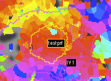
First make a very small ROI for testing. You can make the ROI anywhere, but inside V1 where the retinotopy produced good results would be a good place to start and for the sake of following through on the tutorial you may want to get a similar set of voxels as is shown below:
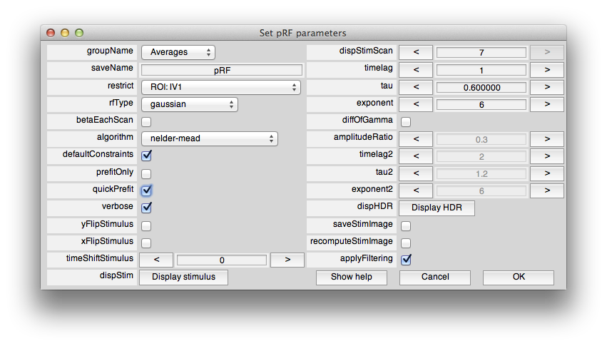
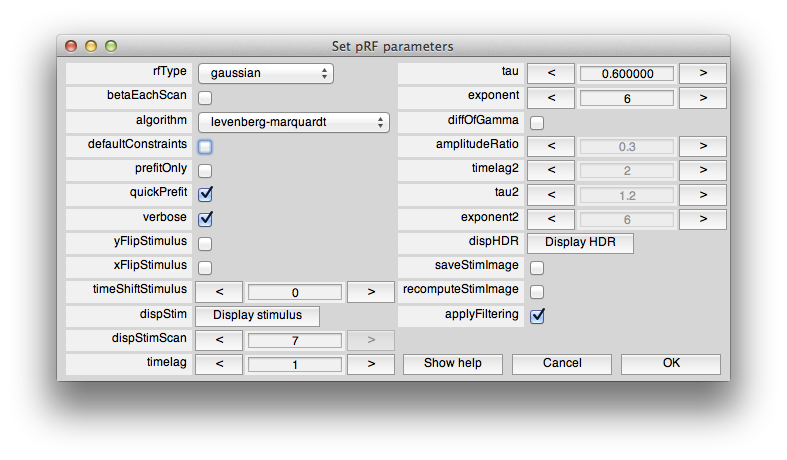
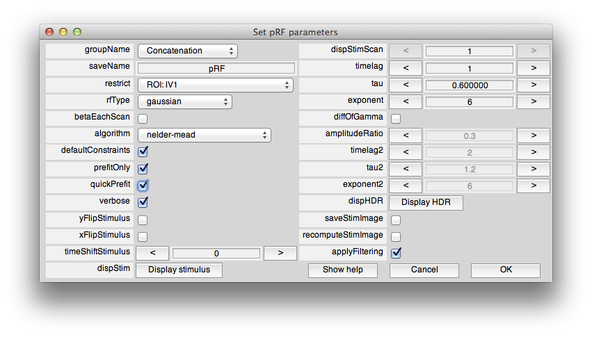
Now, from the Analysis menu select pRF. You should see a dialog box like this:
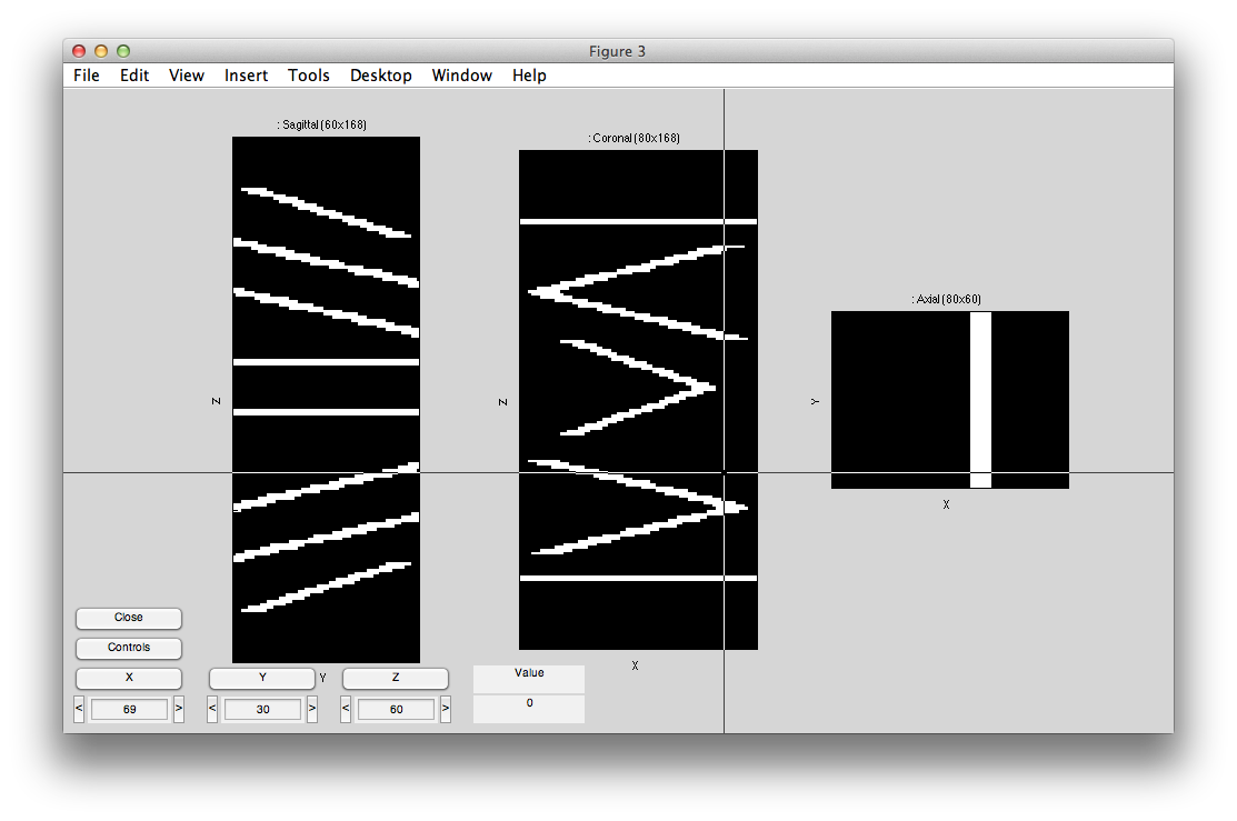
This sets the options for the pRF analysis. The help menu should give explanations for the options, so we will just cover a few things here that are essential to know. The pRF analysis needs to know the stimulus that was presented during the scan. The code retrieves this from the stim file. You can take a look at what it computes as the stimulus by clicking the Display stimulus button. For example, let's look at the stimulus for the 7th scan in Averages (the average of the bar stimulus scans). Set dispStimScan to 7 and click Display stimulus and you should see this (this may not work on a non-mac computer):
What you are looking at is the stimulus with different cuts through a volume with axis x and y (image dimensions) and t (time in Z dimension). So, if you click the Z button you should see what the stimulus looks like animated volume by volume. Note that for our calculations we consider the stimulus to be changing at the same rate as the data acquisition. That is, the stimulus changes position each volume. We are ignoring all of the sliding bars that you see in the stimulus shown above. A more sophisticated analysis might try to take into account every frame of the stimulus and use all of that to generate a pRF model, but here we just think of everything happening within the bar as contrast changes that stimulates a pRF and therefore the stimulus image is just showing areas in white where there was high image contrast and black where there was no image contrast. Click Close to close the stimulus view.
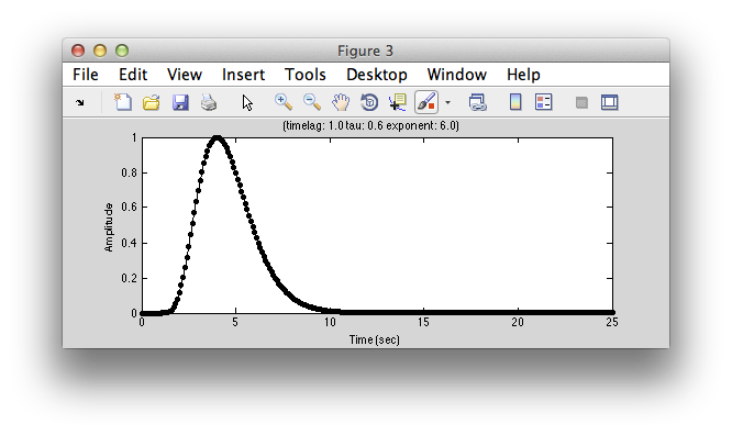
Next, lets take a look at the model hemodynamic response function. Click Display HDR:
You can change parameters of this function by changing the parameters (timelag, tau and exponent). It is simply a gamma function commonly used as a simple hemodynamic response function. If you want an hemodynamic response function that has a negative undershoot, click on diffOfGamma and display again. Usually you don't need to adjust this function, but if you have different assumptions about what a “canonical” hemodynamic response function is you can change parameters to get what you want. Note that the basic fit uses this common hemodynamic function shape and convolves it with the model response time series, you can also fit a hemodynamic function at the same time as fitting the receptive field. This is set by changing the rfType to “gaussian-hdr”. But, for now, let's stick with the basics. We'll get back to more advanced fitting in a little bit.
So, now let's run it. Make sure that “restrict” has the ROI you just created (otherwise it may take a very long time to compute - if you make a mistake and it is running too long, your only option is to hit ctrl-C in the command window, which will crash you out to the debugger, but won't have any other bad side effects). Click OK. Then select Scan 7 (the bars stimuli scan) from the dialog that pops up. At this point you may get a pop-up with the following:
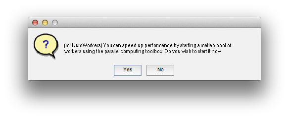
Basically, the algorithm work much faster if you use the parallel toolbox. By clicking Yes (this option may not be available if you do not have access to the parallel toolbox), it will start a number of threads each on a different processor of your machine. This speeds up things since on each processor you can be fitting a different voxel simultaneously. So, generally it is worth saying Yes to this dialog. Note that there appears to be some issue as of this writing (6/18/2013, Mac OS 10.8) with java and the parallel toolbox (the program will crash in matlabpool) that can be fixed by a patch.
It should now be fitting the time series. This can take some time depending on how big the ROI is that you made. You can check the progress in the matlab window.
6. Examining output of pRF analysis
When processing is finished, there should be 4 new overlays loaded (r2, polarAngle, eccentricity and rfHalfWidth). Switch to scan 7 and you should see an r2 map that looks something like this (note that if you click on a voxel within an ROI you may get a different plot - summary of the whole ROI - so either Hide all the ROIs (menu at left) or click on a voxel outside the ROI):
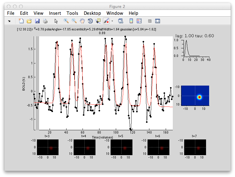
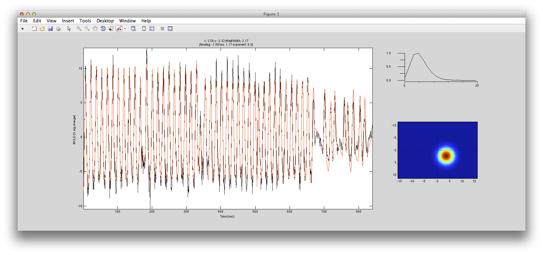
This shows the amount of variance accounted for by the model fit. You can examine the fit by interrogating voxels with the pRFPlot interrogator. To do so, make sure the interrogators are running (Plots/Interrogate Overlay) and make sure that the interrogator pRFPlot is selected in the bottom left of the screen. You may want to make sure that you hide your ROI viewing since clicking on a voxel within the ROI will bring up a different display which shows the fits of all the voxels as explained below. Now go click on a voxel. For example, if you click on the voxel [12 30 22] you should see the following:
What you are looking at is the data in black with the model fit in red. The top right shows the model hemodynamic response function used (which should be the same for all voxels since we did not fit its parameters for this fit). Below that on the blue background is a display of the fitted RF. It appears on the right side of the screen which is a good sanity check since this is the left visual cortex. If you drag your mouse over the time series the gray bar should move. The gray bar is simply depicting the time window being displayed in the black/red images below. What those images are showing is the stimulus at that time (gray bar) with respect to the receptive field for that voxel (red).
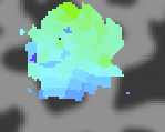
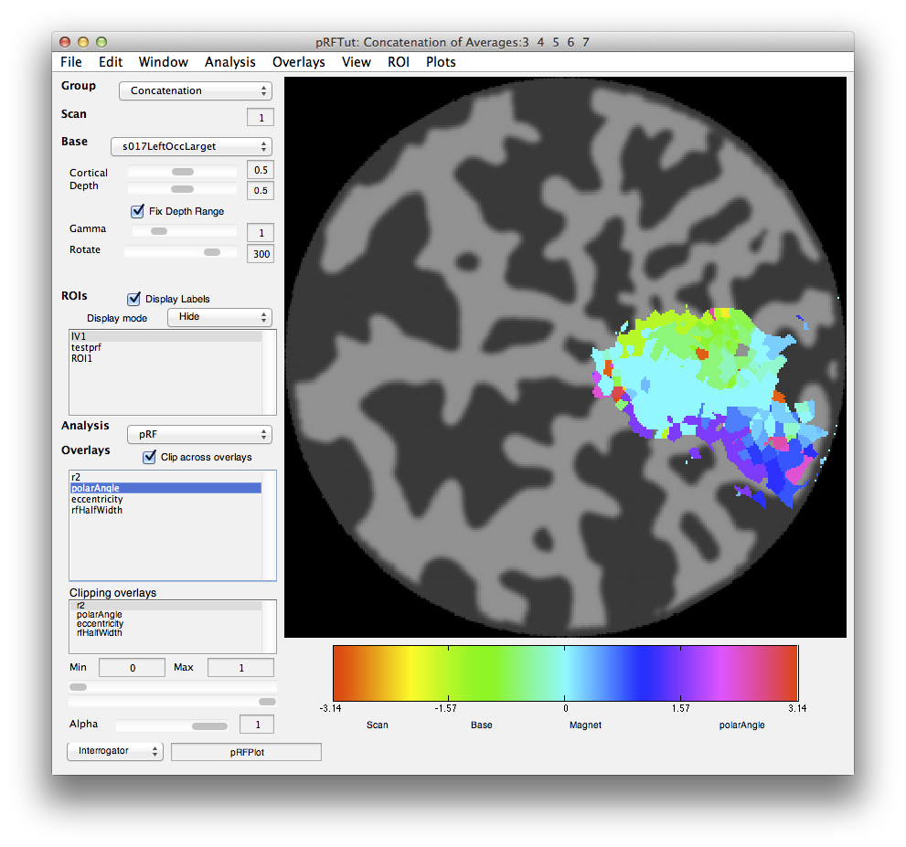
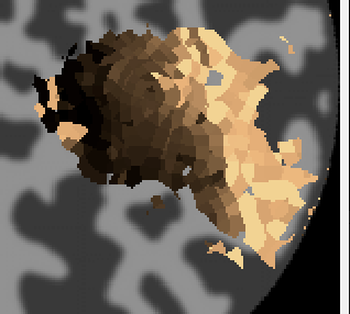
Now let's go back and look at the various other overlays. If you click on the polarAngle overlay you should see the following:
Note that you see a nice gradation as receptive fields are going from the lower right visual quadrant in green to the upper right visual quadrant in blue - just as is expected for the retinotopic ogranization of V1. You should click on individual voxels in green and in blue and be able to see in the interrogator window that the receptive fields are moving as expected. For example here is one from the green region which is more dorsal in V1 and thus responds to the lower visual field:
And here is one from the blue area which is more ventral and thus responds to the upper visual field:
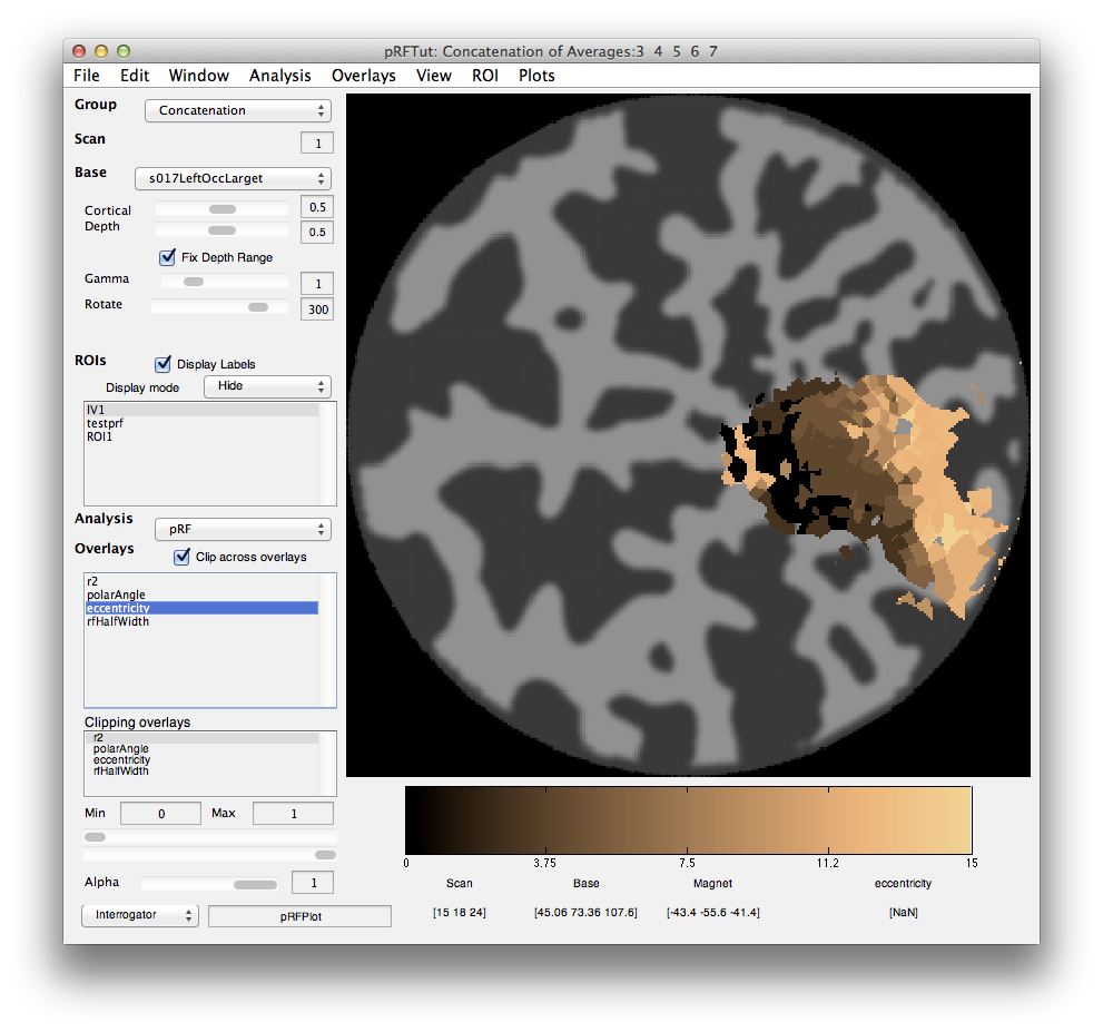
Next click on the eccentricity overlay and you should see the following:
Again a nice gradation as expected from retinotopy. Lighter colors are more eccentric. If you click on voxels at various positions you should see the eccentricity of the RFs.
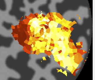
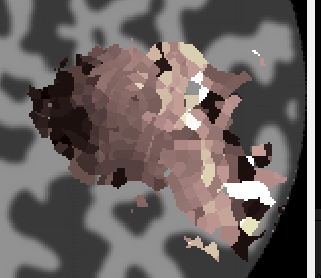
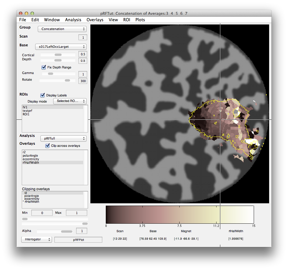
Finally, we can look at the rfHalfWidth. This is the size of the RF and is actually the std of the gaussian used to fit the receptive field. The map should look something like this:
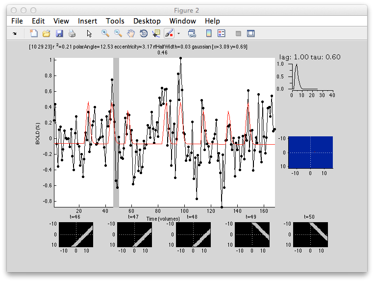
Its a bit noisier in the sense that there isn't as clear a gradation as for eccentricity, but if you squint there is a tendency for RFs that are bigger (lighter colored) to be more eccentric as expected from the known physiology. Note that there are some voxels that are black suggesting very small RFs. These are likely not real but one failure mode of the algorithm. Clicking on one of them (e.g. [10 29 23]) you can see what happened:
What happened is that the algorithm found that it could make the RF really really small and then account for a few time points in the time series (the red spikes you see). Basically what is going on is that for a tiny RF the response are very infrequent and so the algorithm can fit noisy single points in the data. Note that the variance accounted for by this fit is not as good as other voxels, so you can go set the Clipping Overlay r2 to have a minimum of 0.4 (make sure to have “Clip across overlays” checked, then click on the r2 in the Clipping overlays and set the min field), then you will see that all these black voxels are thresholded out:
7. Constrained search
Next we will try and refit the population RF using different options for the fitting parameters to better understand what is going on.
We will explore how to set constraints on the search. For example, the voxels with rfHalfWidth very small are unlikely to be real, so it would be nice to set a constraint on the algorithm to avoid it finding such a small RF.
To do this you can recompute the fits for specific voxels - in particular, choose a voxel that came up black in the pRF analysis rfHalfWidth map. What you need to do is make sure that input focus is on the mrLoadRet window (click on the title bar for instance). Now using the interrogator function, you should click on a voxel while holding the shift key down. (Note that this may not work on a non-Apple machine - if clicking on an individual voxel while shift is held down does not work, then just re-run the whole pRF analysis from the Analysis menu).
Make sure you keep the shift key down until you see the pRF options dialog box come up:
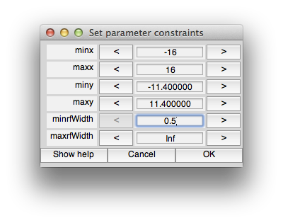
We can now set the constraints so that we don't allow fits with tiny receptive fields. To do this, we have to use the levenberg-marquardt algorithm instead of nelder-mead. This is because levenberg-marquardt is a non-linear minimization algorithm which takes constraints, but nelder-mead simplex method is an unconstrained search. Note that the default is to use nelder-mead because it doesn't seem to get stuck in local minimum as much as levenberg-marquardt. If you want to learn more about these algorithms books like “Numerical Recipes” are a standard reference. So, first we set the algorithm to levenberg-marquaredt. Next unclick “defaultConstraints”. Also click “quickPrefit” (more about that in a minute) and click “OK”. You should see the following constraints dialog come up.
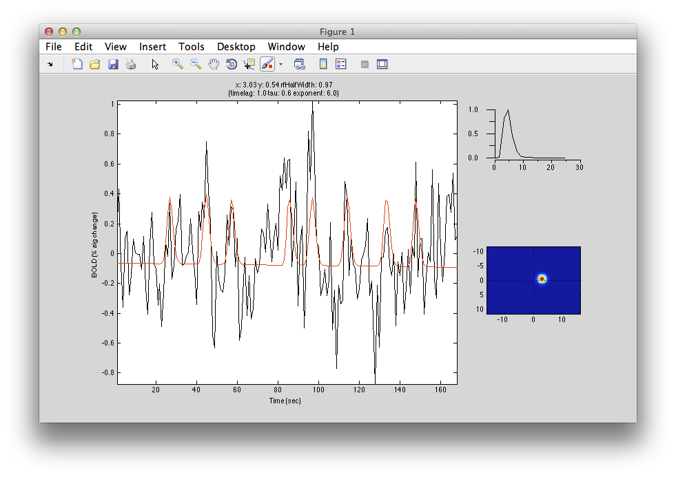
You can set constraints on any of the parameters, but for this case, let's just set the minrfWidth to 0.5 to keep from fitting a very small RF. Set that and click OK. After a minute you should see a window appear in which you can see the progress of the fitting algorithm (it should up-date from time to time with the RF moving around and the red model responses changing).
In this case, it settled on an RF slightly larger than the minimum (0.76) and still seems to have got the right location for the voxel (compare the x,y position with neighboring voxels in the map).
You may want to refit a few voxels and see how changing the constraints in various ways changes the fit that you get.
8. Prefit
When doing nonlinear fits, the starting point of the algorithm often has a large impact on the optimal fit achieved. For example, if the initial estimate of the RF that you give the algorithm is very far away from ideal, the algorithm can get lost in the error space and stuck in a local minimum with parameters far from the global optimal. If you could tell the algorithm where to start - like that you should start in the contralateral visual field for instance, you could do better.
The way we deal with this problem is by computing a grid of model receptive fields at many different locations in the visual field with many different receptive field sizes. We then do a quick test - what we call “prefit” - to see which of these model responses is most highly correlated with the actual voxels responses. By choosing that RFs parameters as the starting point we could do a better fit.
But, how many model receptive fields to calculate? The more you calculate the longer the algorithm takes, but the better the starting estimate. So, there are a few options that you can play with here. Shift-click on a voxel to bring up the pRF parameters dialog box. quickPrefit only computes a small number of model responses. This is useful for testing things out quickly, but the problem is that you may not have sampled the space of RFs very well and so the algorithm later will get stuck in a local minimum. We note that this is particularly true with lavenberg-marquardt which seems to not move very far from the initial starting point. This is why we default to using the nelder-mead even though it cannot do constrained searches.
The other option to note is the “prefitOnly” option. What this does is compute the best RF just based on the prefit (no nonlinear search). It just matches the best model response with the voxel response and reports that as the fit. It is very quick and dirty and can give a pretty good idea of whether things are working or not, but the results will be quantized to only the RF locations and sizes that were computed.
9. Fitting hemodynamic response function
Up to now we have been using a “canonical” hemodynamic response function. In some cases you may want to relax this assumption and actually try to fit the hemodynamic response. Note that when you do this there are more parameters in the model and lots of opportunities to get stuck in local minimum, so the fit gets harder to do. Nonetheless we can try to estimate the hemodynamic response function at the same time. Shift-click on a voxel with very high r2 like [10 31 20]. Now, in the options dialog box, change the rfModel to “gaussian-hdr”. Keep everything else with the default values - in particular, probably best not to do a quickfit since we need good starting parameters. You should see a window like this:
You can watch as the algorithm adjusts both the RF location and the shape of the hemodynamic response function to find the best fit. Here is in example of it doing the fit with the hemodynamic response:
10. Running a full analysis on V1
Ok. Now we are ready to try a bigger ROI for a more real test. To do this, we are going to now concatenate all of our various stimulus types together so that we can use all of the data that we have.
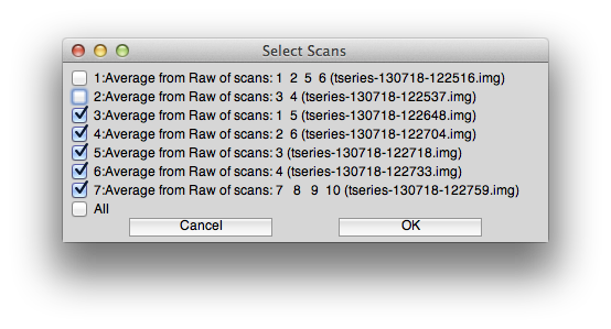
So, go to Analysis/Concatenate Time Series and concatenate scans 3-7 (make sure not to concatenate the scans 1 and 2 which were the ones used to make the standard retinotopy and have the response time series shifted and reversed). You can use the standard options for filtering and the like on the concatenate dialog box. The scans you select should look like this:
Now, switch to the Concatenation group and select Analysis/pRF. Let's do a quick and dirty prefit only to see what things look like. Click “prefitOnly” and “quickPrefit” and make sure that the restrict ROI selected is for your V1 ROI.
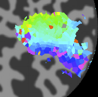
This may take some time to run. Works best if you are using the parallel toolbox and you have lots of free processors! After some time it should complete and you get a rough polarAngle map that should look something like this:
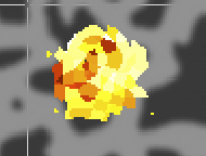
And the eccentricity map should look like this:
Looks reasonable! If you have the processing power and the time to wait, you can try a real fit. Just run pRF from the analysis menu again, but this time use all the default options and click OK. Wait some time and you should get maps that look like the following. Things look generally smoother and cleaner with the exception of a few voxels here and there that are not fit well:
r2 map:
Polar angle:
Eccentricity:
and rfHalfWidth:
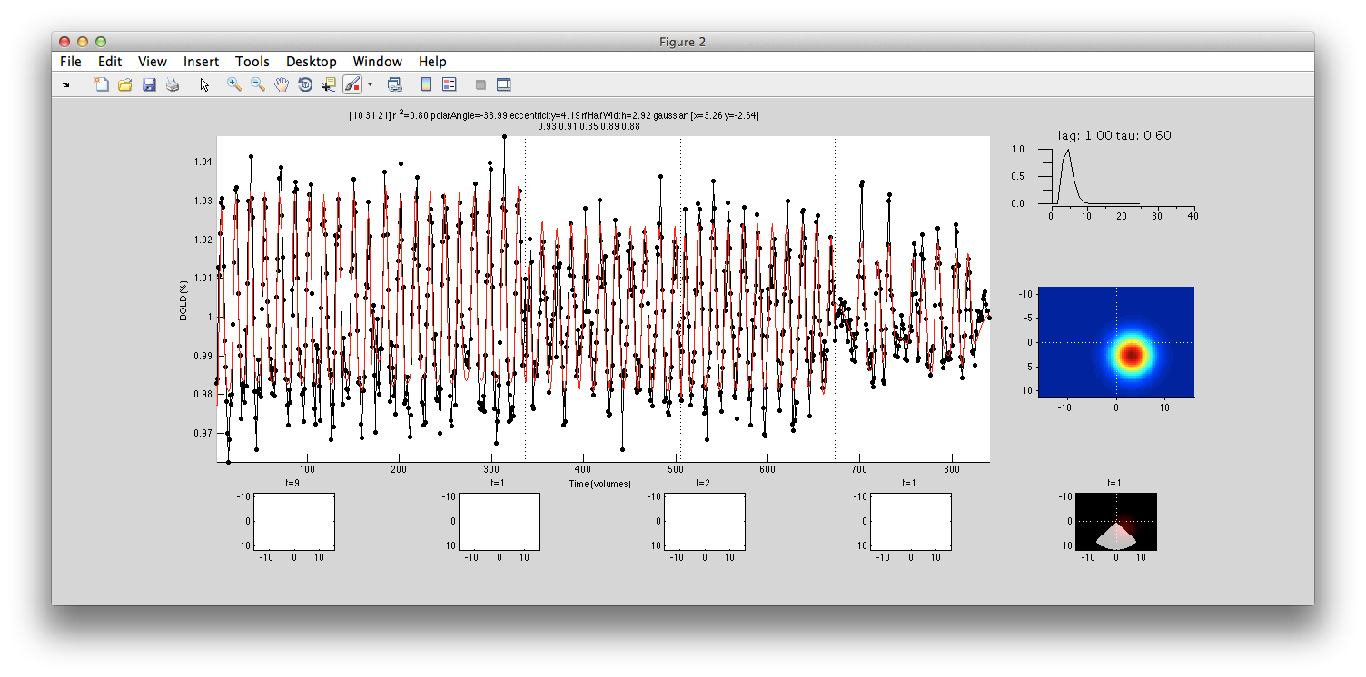
If you click on a voxel (say [10 31 21] that has been well fit with the interrogator, then you should see that it is using the full time course across many experiments and doing a pretty good job of fitting all the data (compare red model curve to data in black). Notice that the overall r2 for this voxel is accounting for 80% of the variance. In individual scans within the cocnat (second row of title), we see that it is account from 85% to 93%.
Finally, if you have the V1 ROI showing and click a voxel within the ROI:
You can examine all the RFs within the ROI together. You should see a figure like the following:
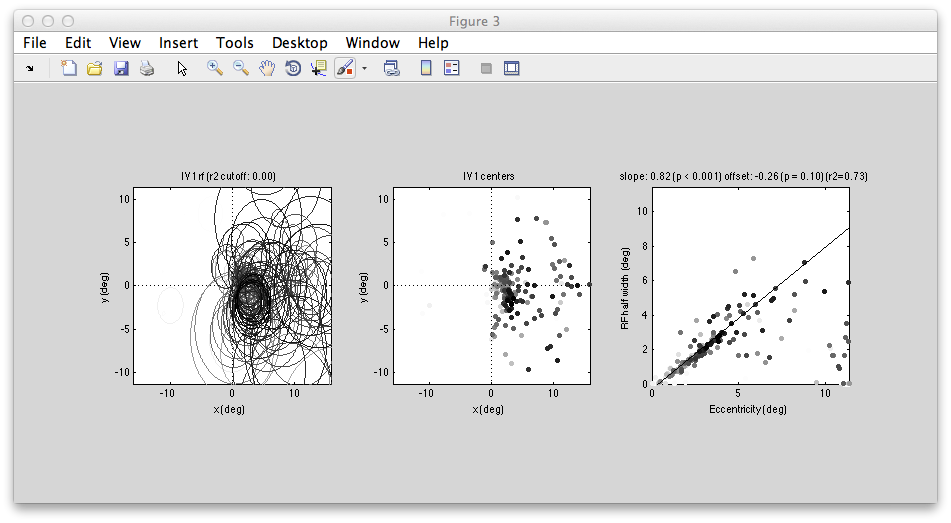
Left shows all the RFs drawn on to the visual field - they all are in the contralateral (right) visual field and look like they do a reasonably good job of tiling that space. The plot of RF half width (std of gaussian receptive field) against eccentricity shows a nice linear relationship which is also what we expect in V1.
-jg.
Classification tutorial overview
This tutorial explains classification analysis with fMRI data using mrTools. Classification analysis can be used to examine distributed patterns of activity - often subtle responses that are hard to examine with other methods. For example, the responses to different orientations which might be distributed across the cortex (see: Freeman et al and Sasaki et al for how they are distributed). Kamitani and Tong showed that you could use classification techniques to read-out the orientation representation. That is, they build classifiers on a subset of data collected as subjects viewed gratings of different orientations and then tested that classifier with a left-out set of data. They were able to show that they could correctly determine what stimulus orientation subjects had been looking at, just by looking at their fMRI measured brain activity. Here we will go through what you need to know to do these types of analysis. The tutorial has one section on basics about classification (not necessarily about fMRI) and another section which uses actual fMRI to do a very simple classification analysis (was a stimulus presented above or below the fixation point?).
You can download the data for the second part here. Its a big file, so it may take some time to download.
You can download the tutorial files from:
Note that this is a rather big file, approximately 430MB.
The files are provided as a tar/zip file. In Mac OS X you should be able to just click to open the files in the Finder. Otherwise, you can go to a terminal and do:
gunzip classificationTutorial.tar.gz
tar xvf classificationTutorial.tar
You should familiarize yourself with the basics of data analysis in mrTools by doing the retinotopy tutorial and the event related tutorial before going through this tutorial.
Finally, you will need to download and put the following matlab functions into your path:
svn checkout http://gru.brain.riken.jp/svn/matlab/classification classification
Some documentation for these functions can be found here.
Classification Basics
Mean classifier
In this first part, we are just going to play around with different classifiers to see how they perform on data to get a feel for the strengths and weaknesses of different methods.
We begin by creating a set of test data. What we want is two sets of data from two different classes. For classification in the context of fMRI data you can think of these as responses generated from two different kinds of stimuli or different kinds of tasks etc. Each dimension is the response (usually the average over some period of time) of a different voxel. For the test data we will create and use data with only two dimensions so that it is easy to visualize and understand what is going on - meaning that it is like using fMRI data from only two voxels. Conceptually, everything should generalize to multiple voxels. But, beware of the "curse of dimensionality" in which adding dimensions increases the volume of the space that one has to search for solutions in - this can occasionally cause problems.
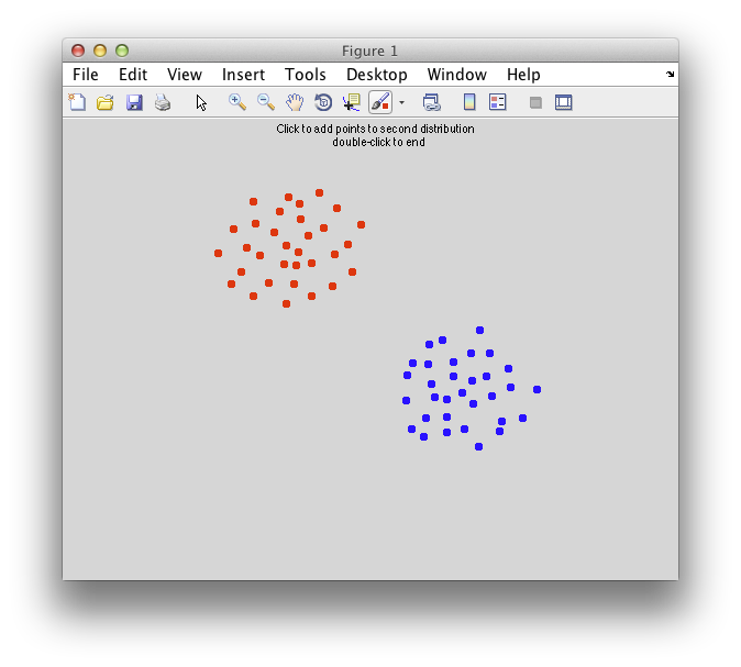
Ok. So let's create the simplest case for a classification. Two data sets that are separated from each other and should therefore be easily classifiable. We will define the points ourselves by using the program classifyTest:
[x1 x2] = classifyTest('type=none');
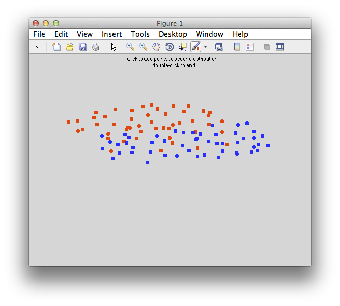
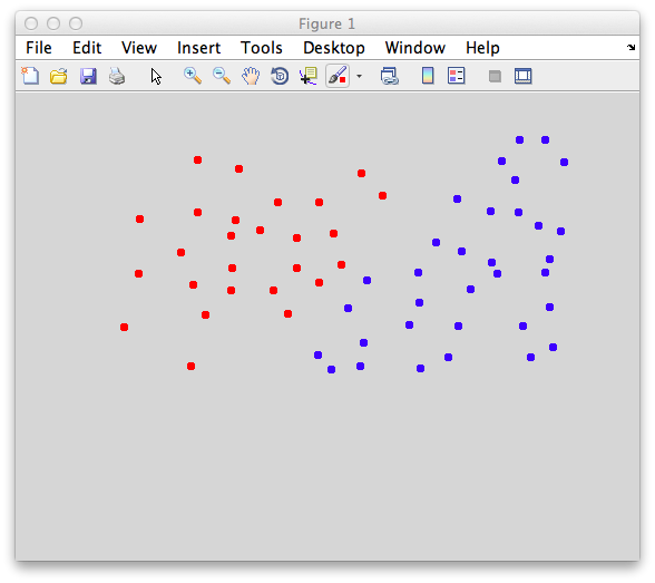
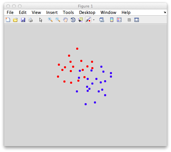
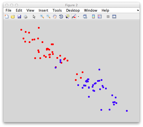
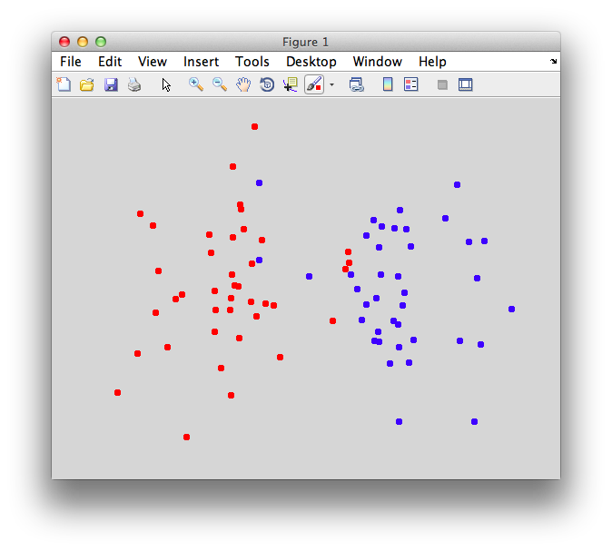
On the graph, click 20 or 30 points roughly in a circle in one location and then double-click the last point. Then make the second set of 20 or 30 points in a location slightly removed. It should look something like this:
Ok. Now in x1 and x2 we should have the coordinates of all the points that we made. You can take a look at them:
>> x1

x1 =

        -0.673963133640553          0.87280701754386
        -0.763824884792627          0.68859649122807
        ...
>> x2

x2 =

         0.383640552995392         0.013157894736842
         0.197004608294931        -0.171052631578947
         ...
Only the first few points have been shown. If you want to use nearly exactly the same data as is shown in this tutorial. Copy and paste the lines in the following to your matlab buffer:
To define some terminology here. We have two classes (red and blue points now named x1 and x2, respectively). Again, classes can be response to different kinds of stimuli (horizontal vs vertical orientation) or different kinds of tasks (adding vs subtracting numbers), anything you like. Each row is an “instance” of a response to each class. It has two columns, which would be the responses of voxel 1 and voxel 2 to that instance.
Linear classifiers are defined by the “projection line”. This is the line (and its a line even if you have more than two dimensions for your data) upon which you project all new instances. Projection means to drop a line from each instance (which is a point in the space) perpendicular to the projection line. The point where this intersects the projection line is called the projection of the point and is also the point that is closest to the instance on the projection line. It is easy to find the projection - you just take the dot product of the vector that defines the projection line and the instance.
Once you find the projection of each instance on to the projection line you compare it against a bias point if it is less than the bias point you are going to say the instance comes from the first class and if it is larger than the bias point it comes from the second class. That's all there is to a linear classifier. Just to repeat, you do the following:
- Get the projection of each new instance on to the projection vector by taking the dot product of the instance and the vector that defines the projection line
- Compare that to the bias point (note that the projection is always a scalar value)
But, how to define the projection line and the bias point. Let's start with the easiest of all classifiers. We will define the projection line as the line that intersects the means of the two class distributions. Let's see what that does. First let's get the mean of both distrubtions:
m1 = mean(x1)
m2 = mean(x2)
We now pass it into classifyTest to have classifyTest classify based on this projection line. Do the following:
classifyTest(x1,x2,'projectionLine',[m1;m2]);
You should see a graph that looks like the following:
Note that there are two lines that are drawn. A white dashed line which is your projection line. Try to visualize what each point would look like if you drew a perpendicular from the white dashed line to each point and placed each point (instance) onto that projection line. There is a solid white line which is the decision boundary it is defined to be perpendicular to the projection line and is centered on the projection line at the bias point (which has been chosen for us as the point in between the two centers of the distribution that we passed in). Note that the decision boundary is in general an n-1 dimensional plane. That is, if we had k voxels instead of the 2 voxels of data in this case, the decision boundary would be a k-1 dimensional plane. The projection line would still be a line. The decision boundary you can think of as a wall that separates points into two different classes.
Ok. That was easy, but what happens if there are overlapped points? Let's make some points that are overlapped:
[x1 x2] = classifyTest('type=none');
You should make points that look overlapped like this:
Again get the means of the two classes to define a simple classifier that simply projects each point on to the line defined by the means:
m1 = mean(x1);
m2 = mean(x2);
classifyTest(x1,x2,'projectionLine',[m1;m2]);
It should look like this:
Note that there are some misclassified points that are marked in x that end up on the wrong side of the decision boundary. Note that this is not a good way to test a classifier since we are testing with the same set of data that we built with - this can cause very serious problems of overfitting - more on that later and how to do cross-validation to avoid these problems.
Bias point
Remember that we said that the linear classifier is just a projection line and that we just use the dot product of the vector that defines that projection line and each instance and compare that to a bias point? Let's go through that step-by-step. We have been defining the classifier according to the projection line that goes through the two means of the distribution and that is what we pass into the function classifyTest. However, what does it mean the vector that defines the line? Well, this is actually meant to specify just the direction of that line which is defined as a vector w as follows:
w = m2-m1
Quite simple, huh? You can pass that into classifyTest to make sure that gives the expected results:
classifyTest(x1,x2,'w',w);
Now, let's talk about the bias point. How do we calculate that? The code has been setting it for you (that is, behind the scenes when you define the classifier weights, a calculation is being made for where the bias point is, and now we are going to compute that ourselves). Its worth understanding what the code does to define this bias point. So, lets just enter an arbitrary bias point that won't work. Like 0:
classifyTest(x1,x2,'w',w,'biasPoint',0);
You should see that the output has the decision boundary in the wrong place and so more instances get misclassified:
To find a better boundary, we can find out where each one of the instances in each distribution project on to the classifier line and then find the midpoint between these two distributions. So, to get the projection we simply take the dot product of the weight vector times each one of the instances;
for i = 1:size(x1,1)
  p1(i) = dot(w,x1(i,:));
end
Note that dot product is simply multiplying each dimension of each instance by the corresponding element of the weight vector and summing over that. That is why we call it a 'weight' vector. The larger the value in w, the more weight is given to the value of that dimension. So, just to be clear, for example dot product for the first instance is calculated as:
firstInstance = x1(1,:);
projection = sum(w(1)*firstInstance(1) + w(2)*firstInstance(2));
The value projection should give you the same value as p1(1). Now, on with computing the best bias point. Lets find the projection of the other class on to the projection line:
for i = 1:size(x2,1)
  p2(i) = dot(w,x2(i,:));
end
Ok. So let's look at the projection values for each class as distributions. Note that this is now one dimensional since it is the scalar values on the projection line. This is the point of the classifier - it turns the k-dimensional (in our case 2D) instances into a one dimensional scalar value which can best distinguish the two classes. Let's look at that:
  figure
  [n binX] = hist(p1);
  bar(binX,n,'FaceColor',[1 0 0]);
  hold on
  [n binX] = hist(p2);
  bar(binX,n,'FaceColor',[0 0 1]);
You should see something like this:
Notice that the distributions are pretty well separated. That's because the classifier is doing a good job of turning our 2 dimensional instances into one dimensional points (the projection onto the projection line) that best separates out the two classes.
Now, to best separate out the two classes, we just need to find a good boundary in this one dimensional space that separates out the two distributions. The center point between the mean of the two distributions will do (assuming equal variance of the red and blue distributions):
mp1 = mean(p1);
mp2 = mean(p2);
biasPoint = (mp2+mp1)/2;
You can draw that biasPoint on to the distributions to see what it looks like:
vline(biasPoint);
You should see that with this bias point you only misclassify a few of the points. To see it in the original space, we can set it in classifyTest:
classifyTest(x1,x2,'w',w,'biasPoint',biasPoint);
Note, now you know all it takes to build and test a linear classifier. To build you need to specify a projection vector (i.e. a weight vector) and the bias point. To test, you take the dot product of a new instance (not in the build set) and the weight vector and compare against the bias point. So, you can classify any instance you want by hand. For example, say the fourth instance in the first class:
testInstance = x1(4,:);
dot(w,testInstance) < biasPoint
This should return true, saying the point is in the first class (unless it happens to be a point that is misclassified). Take another point from the second class and it should return false (again, unless it is misclassified):
testInstance = x2(7,:);
dot(w,testInstance) < biasPoint
Check all the values in p1 and p2:
p1 < biasPoint
p2 > biasPoint
These should be mostly 1 - correct classification (note again that this is not a real test since we are building and testing with the same data set). But, anyway, if you want to compute the percent correct, you would do:
(sum(p1 < biasPoint) + sum(p2 > biasPoint))/(length(p1)+length(p2))
Naive-bayes classifier
So, we've been working with a very simple classifier (projection line in the direction between the two means). When does this fail? Well, for one thing it doesn't take into account different variance in different dimensions of the data. One voxel may have the same mean difference between different classes but be so noisy as to provide no reliable difference compared to a voxel that has the same mean difference but very little variance. We can set up this situation by making up some data using classifyTest:
[x1 x2] = classifyTest('type=none');
Something like this:
Copy and paste the data below if you want to use the exact same data as in the tutorial instead of defining your own points:
Now, let's try the mean classifier:
mx1 = mean(x1);
mx2 = mean(x2);
w = mx2-mx1;
classifyTest(x1,x2,'w',w);
This classifier basically weights both dimensions equally even though clearly there is more variability in the dimension on the abscissa:
So, what's the problem with this solution? Well, if you were to do it by eye, you would probably want the decision boundary to be more horizontal - that is, you would want to ignore the differences in the dimension on the abscissa which have high variability, but weight more the differences in the ordinate which has much less variability. Another way to put that is that you want to weight each dimension by the inverse of its variability. The higher the variability in the dimension the less you want to weigh it. So, let's just do that. First let's calculate the standard deviation each dimension (we do this pooling across both classes):
s = std([x1 ; x2])
You should see that s is larger for the first dimension than the second. That is there is more noise on the first dimension (think voxel) than the second dimension (voxel). So, you should adjust the weights accordingly. That is, make the weight on the first dimension smaller because its standard deviation is larger. To do so, multiply each dimension, by the inverse of the standard deviation.
w = w * 1./s;
Now, let's see if that does a better job:
classifyTest(x1,x2,'w',w);
Better. The decision boundary has now rotated slightly more horizontal and gets the fact that there is less variability in the dimension on the ordinate than the dimension on the abscissa.
This solution which assumes that dimensions do not covary is sometimes called a Naive-bayes classifier. Personally, that name doesn't do much for me. But they say that the “naive” part comes from naive thinking that dimensions don't covary (more in the next section about this) and the Bayes becuase this is a Bayes optimal solution for gaussian distributions with equal variances and no covariance.
Fisher Linear Discriminant
So, incorporating the inverse of the standard deviation is a good idea. But, is this enough? Consider the following case in which there is covariance between the response of the two dimensions. That is the higher the response is in one dimension, the higher the response in the other dimension. This can often happen with fMRI data in which neighboring voxels responses covary:
You may want to copy and paste this data set and try it out yourself:
Let's try the tricks we have in our playbook for dealing with this. First the mean classifier:
m1 = mean(x1);
m2 = mean(x2);
w = m2-m1;
classifyTest(x1,x2,'w',w);
And, we get this:
Terrible! What happened? Well, look at the distribution on the abscissa they have a slight difference with the blue to the left of the red and on the ordinate the red is slightly higher than the blue, so the border is correct for the means, but its missing the dead obvious - it should be tilted up and to the right instead of down and to the left.
Ok. So let's go with trick two in our playbook. Let's scale by the inverse of the variances:
s = std([x1;x2]);
w = w.*(1./s);
classifyTest(x1,x2,'w',w);
And we get:
And that helped us, not one bit. Why? Well the variability in each dimension is about the same so weighting by the variability doesn't change a thing.
So, that gets us to thinking about the defining characteristic here - that the responses in the two dimensions covary. We need to use that fact to define the decision boundary. To do so, let's start by calculating the covariance:
c = cov([x1;x2])
If you take a look at c:
c =
         0.126125531914894          0.11893085106383
          0.11893085106383         0.172812588652482
Note that the values on the diagonal are just the variances in each of the dimensions (compare to what var([x1;x2]) gives you. And the value in the top right (symmetrical with bottom left) is the covariance between the two dimensions. So, how should we use this? Well, before we scaled by the inverse of the variances. Doing essentially the same with the covariance matrix here just generalizes that. So, let's scale the mean classifier with the inverse of this covariance matrix:
w = inv(c) * (m2-m1)';
And, Bam! That does the trick:
classifyTest(x1,x2,'w',w);
Why does this work? Well because it takes into account the means, properly weights it by the inverse of the variances (remember that the variances are on the diagonal of the covariance matrix and it takes into account the covariance of the two dimensions. Turns out this formulation - scaling the mean classifier by the inverse of the covariance matrix - is the right thing to do (in a Bayesian optimal kinda way) to solve any classification problem in which the variables are gaussian distributed with equal variance. It has a name. It's called the Fisher Linear Discriminant (remember that, cause it's a great solution!).
Support vector machine
So, Fisher Linear Discriminant works ideally for identically distributed gaussian data - but are there times when it fails? You, bet! When the distributions are not gaussian. We'll get into one way that the fail (and actually a way that all linear classification schemes fail), but first let's talk about support vector machines.
An alternative to Fisher Linear Discriminant for finding a good decision boundary starts from consideration of what makes a good decision boundary. Well, one might think, a good decision boundary is one such that the distance between that boundary and the points of each of the two classes is maximized. For support vector machines, this is called “maximizing the margin” - the margin being the space around the decision boundary without any points from either distribution. So, what does that look like? Make two distributions like this:
And let's calculate the decision boundary that maximizes the margin with classifyTest:
classifyTest(x1,x2,'type=svm');
And we get this:
If you look at this there is a solid white line (the decision boundary) and the dotted lines neighboring define the margin - the largest distance from that boundary to any point in either distribution. The instances that are contacted by the margins are highlighted with a white border. These instances are called “support vectors” because they are the vectors (i.e. instances) that support the solution. If you changed those two points (like removed them), you would get a different solution to the problem - i.e. a different decision boundary that “maximizes the margin”. Indeed, you could remove any other instances from the distributions, the solution wouldn't change at all. It is only these support vectors that matter. Thus the name.
So, how did we calculate this decision boundary that maximized the margin? Well, you could think of it like this. We could try every orientation and position for the boundary calculate the margin for that decision boundary and then choose the decision boundary that had the largest margin. That would work, but would take a long long time. Instead, there is a clever math solution to this. It turns out you can compute the solution by converting the problem of maximizing the margin into a dual problem which if solved can be converted into the solution you want and then use a well known quadratic programming solution to that problem. So, the solution can be calculated very efficiently. The math is very clever - much too clever for me to explain, but there are a number of good sources if you are interested in learning more (Pattern Classification, Duda, Hart & Stork p. Chapter 5 ; A Tutorial on Support Vector Machines for Pattern Recognition, Christopher J.C. Burges, Data Mining and Knowledge Discovery 2, 121-167 (1998) and An introduction to kernel-Based learning algorithms, Muller, Mika Ratsch Tsuda and Scholkopf, IEEE Transactions on neural networks 12.2 (2001))
One thing that may be a bit mysterious, is, what if there is no margin in that the two distributions overlap, like (make some points like the following):
Well, there is a sort of fudge factor parameter C. The larger that C is the more tolerant the algorithm because. That is, if C is 0, then the solution will fail because it can't tolerate any instance being on the wrong side of the distribution. So, for example, if we set C to 0:
classifyTest(x1,x2,'type=svm','C=0');
We get this - total failure:
If we set C to a positive value, you get a reasonable boundary since it ignore the fact that some of the instances are on the wrong side:
classifyTest(x1,x2,'type=svm','C=100');
Note that it still computes “support vectors” as before, but it ignores the fact that there are other instances within the margin and even on the wrong side.
Play around with changing different C values to see the effect. How would you set this value in practice? Well, you could either just set it arbitrarily to some big number or you could use cross-validation to find an optimal C value on some test set of data.
Now, you should go back and try the svm solution on any of the data that we used before - for many it will end up giving you almost identical solutions as Fisher Linear Discriminant. So, why bother? Well, the real beauty of svm is that you can handle non-linear boundaries.
So, here is a problem that busts any linear classifier including Fisher - the dreaded xor. Xor (exclusive or) is a really, really simple function - just return if one of the inputs is high, but not both. In graphical form, it looks like the following:
This is an xor problem because you have to only accept points into one category (red) if it has a high value (like a 1 for the logical case) in one dimension and a low value (0) in the other dimension, but not if it has two high values (1 and 1) or two low values (0 and 0). An svm classifier fails miserably:
classifyTest(x1,x2,'type=svm')
Why does it fail? Well, basically no matter how you split it, you can't cut a straight line through these points to get everything right. Any linear classifier including Fisher Linear Discriminant will fail.
So, what to do? Well, we need a non-linear boundary of course. But, well, that's hard. So very clever people figured out a simpler solution - just add non-linear combinations of your dimensions to your data and then use the good old linear classifier in this new space to do classification. Huh, what? Well take a look at the following:
This is another version of the xor problem but in 1 dimension. There is no boundary that you can put between these points to correctly classify them all. But, if you just add a second dimension which is calculated as the square of the first dimension, you get a 2 dimensional problem which is now separable:
So, just adding a new dimension (calculated as a square of the first dimension) to your data allows you to use a basic linear classifier to beat the problem. So, we could just add new dimensions to our data by computing squares and so-forth, but then our data would get huge. It turns out for support vector machines (and this is a really nice property) the data only appear in dot products with each other and so instead of calculating non-linear new dimensions you can just transform the dot products and this is really quick and easy to do. So, here is a solution with svm in which we add a squared dimension by using this trick of squaring the dot products of the data:
classifyTest(x1,x2,'type=svm','kernelFun=polynomial','kernelArgs=2','C=1')
Note that we don't actually draw the boundaries for technical reasons, but you can see the cyan/magenta boundary fitting the data we made properly and that there are no points that are misclassified. And, here is the rub. Overfitting. With non-linear classifiers you can easily overfit data by getting boundaries that neatly follow the randomness of the data that you have and not generalize well to new data. Consider the following data:
We can try a funky non-linear classification scheme (in this case instead of polynomial function we use a radial basis function - simply a gaussian function to transform into a new dimension):
classifyTest(x1,x2,'type=svm','kernelFun=radialbasis','kernelArgs=1')
And we get this:
Note the funky boundary evident - is this a good generalization of the data? Probably not. How does one avoid this. Two things. One, avoid non-linear classifiers unless you have a very good reason to believe that your data will need non-linear boundaries (like you know you have data with the xor problem). Second, use cross-validation.
Cross validation
There's not much to say about cross-validation except that you must must do it. Build the classifier on some data (build set) and set and test it on some left out data (test set). You can do this by splitting the data in halves (one half build and one half test). But, sometimes it is better to use more data to build to better fit the weights of the classifier and test on fewer instances. At one extreme you can do a leave-one-out classification (that is, build on all but one instance and test on the remaining instance to see how well you did - then cycle through each one of the instances as the left out test set). Another scheme is to use 4/5 of your data to build and test on another 1/5. Finally, for fMRI data, consider doing a leave-one-run-out cross-validation scheme. This is good because any serial dependencies of responses (due to hemodynamic lag and sluggishness) will not contaminate the test set with the end of the responses to the build set and vice versa.
To run a simple leave-one-out cross-validation on any of the data from above do:
l = leaveOneOut({x1 x2})
This should return this:
leaveOneOut) Class 1 has 14 instances with 2 dimensions
(leaveOneOut) Class 2 has 16 instances with 2 dimensions
(leaveOneOut) fisher classifier produced 90.00% correct and took 3 secs 64 ms

l =

                type: 'fisher'
    classifierParams: [1x1 struct]
          whichClass: {[1 1 1 1 1 1 2 2 1 1 1 1 1 1]  [2 1 2 2 2 2 2 2 2 2 2 2 2 2 2 2]}
       classifierOut: {[1x14 double]  [1x16 double]}
     confusionMatrix: [2x2 double]
             correct: 0.9
          correctSTE: 0.0547722557505166
This shows a few things. One which class each instance got classified into (whichClss field). It also tells the overall % correct (90%). The confusionMatrix tells you how many times each category was classified as the wrong category:
>> l.confusionMatrix

ans =

         0.857142857142857         0.142857142857143
                    0.0625                    0.9375
It shows that 85% of the time category 1 was classified as category 1 and 94% of the time category 2 as category 2. Category 1 was classified 14% of the time as category 2 and category 2 was classified as category 1 6% of the time.
Classification on example fMRI data
Now we are going to try to do a basic classification analysis on some real data. For didactic purposes this is going to be a really easy classification - whether a stimulus was presented below or above the fixation point. The experiment was a simple localizer in which different visual stimuli (it is not important for the purposes of this tutorial to know more about what exactly these stimuli were) were presented above or below the fixation point in blocks of 16.2 seconds in a randomized order. The classifier will be build on some subset of the trials and tested on the left out portion - to see if we can predict which location the stimulus was presented on these test trials.
Now, typically, you may want to run classification analyses on more subtle differences, particularly responses that you think have distributed representation hard to get at with other means, but we will use this example just to get used to the basics of the analysis. Based on the topographic representation of space in visual cortex it should be very easy to find some voxels that respond more when the stimulus is above the fixation point and some voxels that respond more when the stimulus is below the fixation point. Combining the information from all these voxels using classification it should be very easy to predict where the sitmulus was presented.
Event-related analysis
Switch directories to the classification tutorial (classTut) and start mrLoadRet:
cd classificationTutorial;
mrLoadRet;
First, we're going to run a basic event-related analysis. You may want to review the event-related tutorial. Start by concatenating together all the scans using Analysis/Concatenate Time Series. Default parameters for the filtering are fine.
Switch to the new Concatenation group (Group drop down on top left) and check the scan info Edit/Scan/Info (⌘I). Just make sure that you correctly concatenated the four scans (scanList=[1 2 3 4]) and used the default filtering options (filterType = “Detrend and highpass” filterCutoff = 0.01)
Now run an event-related analysis (Analysis/Event Related Analysis) and use all the default options until you get to the following dialog box in which you will set the varname to upDown (Note that it is really important to put the variable name “upDown” into the dialog box otherwise it won't know what variable to compute event-related analysis for):
Set the Clipping overlay Min (slider or text box in bottom left) to 0.2) and then switch the Base (drop-down in top left) to display the left occipital cortex flat patch (s017LeftOccSmall). You should see a map of the r2 values that looks like the following.
Turn on the interrgator (Plots/Interrogate Overlay) and click on a few points in the top using the eventRelatedPlot and you should see something like this:
Clearly larger responses for the trials when the stimulus was in the lower visual field, just as is expected for the topographic representation in early visual cortex. Clicking on voxels at the bottom, you should see this pattern reversed.
Classification analysis
Now, it should be quite easy to build a classifier, right? Just by seeing whether voxels that represent the upper visual field are responding or the ones that represent the lower visual field are responding we should be able to predict where the stimulus was. Let's train a classifier to do this.
We need to get the instances of responses for each stimulus type. That is, we want a number representing the response to each trial from each voxel in an ROI. Let's do this for the left V1. Load the lV1 ROI from File/ROI/Load
You should see the ROI like this (check that Selected ROIs (Perimeter) is selected in the Display Mode drop down in the middle left.
Note that the voxels with high r2 are right at the top and bottom of V1 just as expected (since that is where the lower and upper visual meridians are represented).
Now go to the Matlab command line and use getStimvol to get the stimvols for the upDown stimulus. That is, we want to know which volumes in the scan each stimulus began at. That is what is put into stimvol. Stimvol is a cell array with two elements. The first is all the stimvols for when the stimulus was in the upper visual field, and the second when the stimulus was in the lower visual field.
>> stimvol = getStimvol(getMLRView,'upDown')
(getStimvolFromVarname) taskNum=[1], phaseNum=[1], segmentNum=[1]
(getStimvolFromVarname) upDown=1: 10 trials
(getStimvolFromVarname) upDown=2: 10 trials
(getStimvolFromVarname) taskNum=[1], phaseNum=[1], segmentNum=[1]
(getStimvolFromVarname) upDown=1: 10 trials
(getStimvolFromVarname) upDown=2: 10 trials
(getStimvolFromVarname) taskNum=[1], phaseNum=[1], segmentNum=[1]
(getStimvolFromVarname) upDown=1: 10 trials
(getStimvolFromVarname) upDown=2: 10 trials
(getStimvolFromVarname) taskNum=[1], phaseNum=[1], segmentNum=[1]
(getStimvolFromVarname) upDown=1: 10 trials
(getStimvolFromVarname) upDown=2: 10 trials

stimvol =

    [1x40 double]    [1x40 double]
This shows you that there were 10 trials of each in each of the four component localizer scans for a total of 40 instances of each response type.
Now that we know the stimvols we need to get the responses to each stimulus presentation. We are going to do this by averaging the response in the time series for each of the voxels in left V1 across the time when the stimulus was presented (actually we time shift by a few seconds to account for the hemodynamic lag). First load the time series for lV1:
>> lV1 = loadROITSeries(getMLRView,'lV1')
(loadROITSeries) Loading tSeries for lV1 from Concatenation: 1 took 0 secs 766 msmin 00 sec)

lV1 =

         color: 'magenta'
        coords: [4x5397 double]
          date: '05-Jul-2013 12:57:25'
          name: 'lV1'
         notes: ''
     sformCode: 1
      viewType: 'Volume'
       vol2mag: [4x4 double]
       vol2tal: []
     voxelSize: [1 1 1]
         xform: [4x4 double]
       scanNum: 1
      groupNum: 2
    scanCoords: [3x200 double]
             n: 200
       tSeries: [200x480 double]
Now in the field tSeries you have the time series (480 volumes) for each of the 200 voxels that we have in left V1. We next set a sort order. This is used in times when you are only going to use a subset of your voxels in the classification (for example, you may want to use only a one hundred not the full two hundred to equalize ROI size across idfferent visual areas). But, which voxels to use. The sort index tells the programs what order to use. For right now, we don't care cause we are going to use all the voxels in the ROI, so let's just set this to the order the voxels happen to be in the ROI:
lV1 = getSortIndex(getMLRView,lV1);
We now need to snip this up into the pieces of response after each stimulus presentation and average for the duration of the stimulus. We use getInstances:
>> lV1 = getInstances(getMLRView,lV1,stimvol,'n=inf')
(getInstances) Creating 40.0 instances for lV1 with Inf voxels by taking mean from vol 1:6 (2.70s-16.20s) took 2 secs 174 msmin 00 sec)
took 2 secs 174 ms

lV1 =

    [1x1 struct]
Note that getInstances turned lV1 into a cell array (usually we run in on multiple ROIs, so let's just turn it back into a single ROI:
lV1 = lV1{1};
Now, we can grab the instances from the ROI which is stored under the classify field:
>> i = lV1.classify.instances

i =

    [40x200 double]    [40x200 double]
So there are 40 instances of response for each category (stimulus up or stimulus down) and each instance is a 200 dimensional vector (1 dimensional for each voxel - compare to above where we just had 2 dimensions).
Well, we can just run leaveOneOut on this and see how we do:
>> leaveOneOut(i)
(leaveOneOut) Class 1 has 40 instances with 200 dimensions
(leaveOneOut) Class 2 has 40 instances with 200 dimensions
(leaveOneOut) fisher classifier produced 91.25% correct and took 10 secs 449 ms

ans =

                type: 'fisher'
    classifierParams: [1x1 struct]
          whichClass: {1x2 cell}
       classifierOut: {[1x40 double]  [1x40 double]}
     confusionMatrix: [2x2 double]
             correct: 0.9125
          correctSTE: 0.0315918798902503
91% correct is not bad. Note that this is defaulting to using fisher linear discriminant.
So, great. We can classify the stimulus what does that mean? Well it means that there are responses that are specific to whether the stimulus was presented above or below just as expected.If there was nothing useful, this number would hover around 50% and you would know that there probably is nothing very interesting in your data with respect to the variables you are trying to classify.
Weight maps
It is a good idea for any classification you do, to check to see what the spatial arrangement of voxels is that allows the classifier to work. Let's look at this. First lets prepare the ROI by setting its sortIndex (more on this later - but, for now we just set dummy values)
>> weightMap = getClassifierWeightMap(getMLRView,lV1,stimvol);
(getInstances) Creating 40.0 instances for lV1 with Inf voxels by taking mean from vol 1:6 (2.70s-16.20s) took 2 secs 114 msmin 00 sec)
took 2 secs 114 ms
(buildClassifier) Building fisher classifier for ROI lV1 took 0 secs 105 msmin 00 sec)
What this did was build a classifier to classify the stimulus classes in stimvol using all the voxels in the ROI (no cross-validation) and it returns the weightMap.
Now weightMap contains the map of weights for each voxel in the ROI (actually it has the same dimensions as the scan 64x64x38 where values with a weight calculated are set to that weight and all other values contain NaN).
Now let's display it: First drop the erAnal analysis that you are currently viewing by doing View/Remove Analysis. Now from the command line do:
mrDispOverlay(weightMap,lV1.scanNum,lV1.groupNum,getMLRView,{'up vs down'},'colormapType','normal','cmap',splitcmap,'range=[-9 9]','clip=[-9 9]');
You should see the following:
You should see that negative weights are near the top and positive weights near the bottom. This is exactly what we expect based on the topography. Voxels that have a larger response for the stimulus when presented at the bottom have negative weights and voxel with larger responses for when the stimulus was presented at the top have positive weights. You can see this more clearly, but clipping out all the weights that are in the middle ranges. This is done by crossing the min/max ranges of the Clipping Overlay (bottom left). That is, set the min to 0.5 and the max to -0.5 and you should see the following:
Clearly the voxels that have high weights (contribute information to the classifier) are all just where we expect them to be at the upper and lower parts of V1 that represent the vertical meridians where the stimuli were places.
Number of voxels by accuracy plots
Sometimes it is interesting to know how much better performance of the classifier gets as a function of how many voxels enter the analysis. If only a few voxels are needed it suggests strong selectivity - if you need many it suggest weak selectivity in a large distributed pattern. If you add too many voxels you might just be adding noise and performance can decline. So, let's see what happens with this data set.
First we have to decide what order to include voxels in the analysis. This is a very important step. Typically what we do is use an independent localizer of some sort (perhaps retinotopy) to define which voxels we think will have a stimulus driven response. In this case, we are going to cheat a little and use the r2 from the event-related responses. This is cheating because it is a violation of cross-validation (choosing which voxels to use on data from the test set) - we should really choose voxel using data only from the training set or better yet a completely independent data set so that we don't break cross-validation.
But, with that in my mind, we need to get the r2 values from the event-related analysis. Going to the GUI and remove the mrDispOverlay analysis of the classifier weights (View/Remove Analysis). Now go load the erAnal analysis File/Analysis/Load load erAnal/erAnal.mat
Then from the command window get the r2 values of the overlay:
r2 = viewGet(getMLRView,'overlayData',1);
Now we are going to set the sort order according to this r2 map (remember before we just set the sort order to the random order that the voxels happen to be in the ROI):
lV1 = getSortIndex(getMLRView,lV1,r2);
Now, let's compute leaveOneOut classification performance as a function of how many voxels we use. This may take a few minutes to compute:
voxNums = [1:20:lV1{1}.n];
correct = [];
for nVox = voxNums
  lV1 = getInstances(getMLRView,lV1,stimvol,'n',nVox);
  instances = lV1{1}.classify.instances;
  l = leaveOneOut(instances);
  correct(end+1) = l.correct;
  disp(sprintf('%0.2f%% correct with %i voxels',100*correct(end),nVox));
end
Now if we plot it, we can see that basically we always get the best performance even if we use 1 voxel!
plot(voxNums,correct,'ko-');
xlabel('Number of voxels (n)');
ylabel('Classification accuracy (percent correct)');
Just to prove that the order matters, let's reverse the sortindex so that now the worst voxels (in terms of how much they respond to the stimulus - not necessarily how well they differentiate between stimuli) are first.
lV1{1}.sortindex = fliplr(lV1{1}.sortindex);
Now do the classification again:
 voxNums = [1:2:10 20:10:100 120:20:lV1{1}.n];
correct = [];correctSTE = [];
for nVox = voxNums
  lV1 = getInstances(getMLRView,lV1,stimvol,'n',nVox);
  instances = lV1{1}.classify.instances;
  l = leaveOneOut(instances);
  correct(end+1) = l.correct;
  correctSTE(end+1)
end
Now you only get good performance when you add the best voxels back.
plot(voxNums,correct,'ko-');
xlabel('Number of voxels (n)');
ylabel('Classification accuracy (percent correct)');
Classify by hand
Just for fun, let's see if we can classify the data by hand. Let's get the instances again for two voxels:
lV1 = getSortIndex(getMLRView,lV1,r2);
lV1 = getInstances(getMLRView,lV1,stimvol,'n=2');
instances = lV1{1}.classify.instances;
Now we can plot the points:
classifyTest(instances{1},instances{2},'tightAxis=1','type=none')
And we can try the mean classifier:
m1 = mean(instances{1});
m2 = mean(instances{2});
w = m2-m1;
classifyTest(instances{1},instances{2},'tightAxis=1','w',w);
Already that does well. As an exercise try it with naive-bayes or fisher or svm and see what you get.
We can also try to build with all 200 voxels:
lV1 = getInstances(getMLRView,lV1,stimvol,'n=inf');
instances = lV1{1}.classify.instances;
But then it is hard to visualize all 200 dimensions so we need to project into a smaller space. We could do this in many ways. Some people do this as a first step to classification to get rid of noise, but its risky. Which dimension is the best dimension for classification? It could be dimensions that have the most variance in them - but that variance may not be associated with responses that are different for different categories. Nonetheless, we project onto these dimensions - the ones that account for the most variance in the data. We can do this by using PCA:
pcaBasis = pca([instances{1};instances{2}]);
This is essentially a rotation of the data space so the orthogonal axis point in directions of most variance within the data. We take the top two dimensions and project our data down on to those dimensions:
for iNum = 1:40
  x1(iNum,1) = dot(instances{1}(iNum,:),pcaBasis(:,1)');
  x2(iNum,1) = dot(instances{2}(iNum,:),pcaBasis(:,1)');
  x1(iNum,2) = dot(instances{1}(iNum,:),pcaBasis(:,2)');
  x2(iNum,2) = dot(instances{2}(iNum,:),pcaBasis(:,2)');
end
Then the data in these two dimensions look like this:
classifyTest(x1,x2,'tightAxis=1','type=none')
And classifying using Fisher like this:
classifyTest(x1,x2,'tightAxis=1','type=fisher')
We get:
-jg.
The following are some introductory lines to the functionality of the mrLoadRet-4.5 Graphic User Interface. All options in this section will either generate a .mat file, modify mrSESSION.mat or the .img files.
File Menu
Look in the file menu for functions that let you load / save anatomy files, analyses, ROIs and so on. There are also functions that let you print the currently displayed image, import / export data, ROIs, write out information about the session in a Readme.txt file, and quit the current session of mrLoadRet.
Base Anatomy
- Load: Select an anatomy file on which overlays will be rendered. Normally, this will be your inplane anatomy file which was collected during the scanning session at the same slice locations as your functional data.
- Load from volume directory; Select a volume anatomy file on which overlays will be rendered. By default, the file dialog window opens in the volumeDirectory folder specified in your preferences. Make sure that the qform and sform matrices of the file you select are correct. Normally, you will use the volume anatomy file that was used as the target in your alignment steps (see mrAlign documentation).
- Use current scan Lets you use the current functional scan as the background image. You will be prompted to select a time point from the 4D volume; the first frame in the sequence is 1. If you select time point '0', the mean 3D image across time will be used.
- Load flat Load flat patches created by the steps described in the
- Load Surface Load OFF surfaces created with TFI/SurfRelax. You will be prompted for an outer surface filename. Provide the gray matter (GM) surface from one subject/hemisphere. You will then be prompted to select the matching inner surface (white matter, WM), curvature, and anatomy file. See documentation for mrSurfaceViewer for more details.
- Save Save the currently used anatomy image with a default filename
- Save As… Save the currently used anatomy image and specify a filename
Analysis
- Load Load an analysis that was computed and saved earlier. Standard analyses that can be created by functions accessible in the GUI Analysis menu are Time Series Statistics (e.g. mean, median, across time), Correlation Analysis (standard Fourier-based analysis), Event related analysis, and GLM analysis (generalized linear models to produce statistical parametric maps).
- Save Save the currently selected analysis.
- Save All Save all analysis that have been opened in this session.
Overlay
ROI
Import
- Group
- Time Series
- Overlay
Export
- Anatomy
- Time Series
- Overlay: This function exports the current overlay into a NIFTI file. If a flat map is loaded, the user is asked how many different depths should sample the cortex. If she selects 10 for example, and the flat maps are 384 by 384, the flat map will be exported as a 384*384*10 volume, and each slice will be a different cortical depth.
- ROI
- Image
Write Readme.txt
Save mrSession
Quit
Edit Menu
Edit mrSession
Edit details of the scanning session such as a description, the subject id, operator, magnet and pulse sequence. Those were usually when running mrInitRet or mrInit.
Group
Manipulate groups (such as Raw, MotionComp, and Averages
- New Group - create a new group
- Delete Group - delete an existing group, e.g. if you realize that there were some mistakes in averaging across scans, you can delete the group Averages. The function will clean up the appropriate entries in the view variable that goes along with your session.
- Edit Group - This allows you to edit details for each scan in a Group: the scan description, the total number of frames and the junk frames (also called 'dummies') at the beginning of each scan that get disregarded in any analysis.
- Info - show information about each scan in each the current group. For the Average group, this will also show you which files contributed to each average. This is quite an important tool for debugging and checking your analyses.
Scan
Base Anatomy
Analysis
Overlay
- Edit Overlay
- alphaOverlayExponent: this value can be positive or negative. alphaOverlayExponent specifies how much the alphaOverlay masks the selected overlay. With positive value, low values in the alphaOverlay mask more than high values. With a negative exponent, it's the reverse. This is useful for masking overlays with p-value overlays (you want high values to mask more).
ROI
Preferences
Edit important preferences that affect the overall behavior of mrLoadRet. You will see a menu like the following:
| preference | value |
|---|---|
| Site | (e.g. NYU, RIKEN, RHUL, Nottingham, …) |
| verbose | Yes if you want to have messages and waitbars displayed as dialogs, No to have information printed to the terminal |
| interpMethod | Type of interpolation to use. Normally this is set to nearest for nearest neighbor interpolation – on a flat map you will be able to see a crystalline pattern of how the voxels are getting warped. If you prefer a smoother looking overlay, try setting this to linear |
| maxBlocksize | Size of chunks of data to analyze at a time. If you are running out of memory, set lower. A good starting point is 250000000. If you are using 64 bit Matlab (there is a beta which works with mrLoadRet for Mac OS X), set this to a very high number. |
| volumeDirectory | The directory to default to when you load base anatomies from the VOlume directory |
| overwritePolicy | Method to use when analysis is going to overwrite an existing file |
| niftiFileExtension | Nifti file extension, usually .img but can be set to single file .nii |
| selectedROIColor | What color to use to draw the selected ROI. |
| roiPolygonMethod |
Which should be info that you can check in a script.
Finally, let's change the description of the averaged scans. Note that the two averaged scans should be the last two scans in the Average group (i.e. nScans-1 and nScans):
nScans = viewGet(v,'nScans','Averages');
scanParams = viewGet(v,'scanParams',nScans-1,'Averages');
scanParams.description = sprintf('Wedges: %s',scanParams.description);
v = viewSet(v,'scanParams',scanParams,nScans-1,'Averages');
scanParams = viewGet(v,'scanParams',nScans,'Averages');
scanParams.description = sprintf('Rings: %s',scanParams.description);
v = viewSet(v,'scanParams',scanParams,nScans,'Averages');
Finally, save the session to make sure that the changes above stick
saveSession
6. Correlation analysis
You can script the correlation analysis by first changing to the Averages group and then getting parameters:
v = viewSet(v,'curGroup','Averages');
[v params] = corAnal(v,[],'justGetParams=1','defaultParams=1');
Then set the parameters appropriately:
params.recompute(:) = 1;
params.ncycles(:) = 10;
Now run the corAnal
corAnal(v,params);
Finally, if you are done using the view variable, remember to delete it.
deleteView(v);
There. We are done. You have now done the same analysis as you did using the GUI in the retinotopy tutorial. You can now run mrLoadRet and view the results in the same way as you did with the tutorial. After you open up the mrLoadRet viewer, make sure you are switched to the Averages Group and use File/Analysis/Load to load the corAnal/corAnal.mat.
7. Getting data
Getting overlay values
Instead of running the GUI you may actually just want to grab the coherence, amplitude and phase data from the analysis for your own analysis program. You can do that by getting the information from a view variable. You can either use the view variable you were using above, or start a new one:
v = newView;
Now switch to the Averages group and find the wedges scan:
v = viewSet(v,'curGroup','Averages');
wedgesScanNum = viewGet(v,'scanNumFromDescription','Wedges');
v = viewSet(v,'curScan',wedgesScanNum);
Load the computed corAnal analysis in:
v = loadAnalysis(v,'corAnal/corAnal.mat');
Let's get the phase overlay:
overlayNames = viewGet(v,'overlayNames');
phOverlayNum = find(strcmp('ph',overlayNames));
v = viewSet(v,'curOverlay',phOverlayNum);
phOverlay = viewGet(v,'overlayData',wedgesScanNum);
phOverlay now is a 64x64x27 matrix that contains the phase value for every voxel in the volume.
Make sure to remember to delete your view when done:
deleteView(v);
Getting overlay image
You can also get an overlay image like the one displayed in the viewer, without having to interact with the viewer GUI. To do this, start up MLR:
mrLoadRet([])
The empty brackets makes it forget previous settings. Now, change the group and scan to the wedges scan like before, but instead of using a view you created, use the MLR view that is returned by getMLRView:
viewSet(getMLRView,'curGroup','Averages');
wedgesScanNum = viewGet(getMLRView,'scanNumFromDescription','Wedges');
viewSet(getMLRView,'curScan',wedgesScanNum);
Load the analysis
loadAnalysis(getMLRView,'corAnal/corAnal.mat');
Load the right_occipital anatomy:
loadAnat(getMLRView,'right_occipital.hdr');
Set the overlay to ph
overlayNames = viewGet(getMLRView,'overlayNames');
phOverlayNum = find(strcmp('ph',overlayNames));
viewSet(getMLRView,'curOverlay',phOverlayNum);
Now refresh the MLR display and grab the image
img = refreshMLRDisplay(viewGet(getMLRView,'viewNum'));
ok, now display
figure;
image(img);
axis square;
axis off;
And you should get this:
To close the viewer:
mrQuit(0);
Event Related Tutorial (scripting)
This shows you had to do all the analysis form the Event Related Tutorial without the GUI. Note that you may also want to set your verbose setting in Edit/Preferences to 'No' so that all messages and waitbars get printed out at the command line rather that in a dialog.
Overview
- Download the tutorial files
- Concatenate scans together
- Set stimfiles
- Run event-related analysis
- Extracting data
1. Download
You can download the tutorial files from:
Note that this is a rather large file. Approximately 300MB.
The files are provided as a tar/zip file. In Mac OS X you should be able to just click to open the files in the Finder. Otherwise, you can go to a terminal and do:
gunzip erTutorial.tar.gz
tar xvf erTutorial.tar
We assume that you have mrTools running on your system.
2. Concatenate
Start matlab and cd into the erTutorial directory:
cd erTutorial
We will concatenate the scans from the motion group together:
v = newView;
v = viewSet(v,'curGroup','MotionComp');
nScans = viewGet(v,'nScans');
[v params] = concatTSeries(v,[],'justGetParams=1','defaultParams=1','scanList',[1:nScans]);
At this point, the params should look like:
  >> params

params =

                     groupName: 'MotionComp'
                  newGroupName: 'Concatenation'
                   description: 'Concatenation of MotionComp:1  2  3  4  5'
                    filterType: 1
                  filterCutoff: 0.01
                 percentSignal: 1
          projectOutMeanVector: 0
                     paramInfo: {1x7 cell}
                      scanList: [1 2 3 4 5]
                          warp: 0
              warpInterpMethod: 'nearest'
    projectOutMeanVectorParams: [1x1 struct]
                   tseriesFile: {1x5 cell}
We could change any of the parameters that we want at this point, but there is no need, so we will just start the concatenation here:
v = concatTSeries(v,params);
3. Set stimfiles
Here, we write a snippet of code to set all the stimfiles:
nScans = viewGet(v,'nScans','Raw');
for iScan = 1:nScans
  stimfilename = sprintf('stimvol%02i.mat',iScan);
  viewSet(v,'stimfilename',stimfilename,iScan,'Raw');
end
And then check to see if it looks correct
>> groupInfo('Raw')
1: directions/coherences
   Filename: 11+cbi_ep2d_bold_recon.img GroupName: Raw
   StimFilename: /Volumes/drobo/data/nyu/erTutorial/Etc/stimvol01.mat
   junkFrames=[0] totalJunkedFrames=[0]
   voxelSize=[3.0 3.0 3.0] TR=1.2000 Dims: [64 64 22] Volumes=375
2: directions/coherences
   Filename: 12+cbi_ep2d_bold_recon.img GroupName: Raw
   StimFilename: /Volumes/drobo/data/nyu/erTutorial/Etc/stimvol02.mat
   junkFrames=[0] totalJunkedFrames=[0]
   voxelSize=[3.0 3.0 3.0] TR=1.2000 Dims: [64 64 22] Volumes=375
3: directions/coherences
   Filename: 13+cbi_ep2d_bold_recon.img GroupName: Raw
   StimFilename: /Volumes/drobo/data/nyu/erTutorial/Etc/stimvol03.mat
   junkFrames=[0] totalJunkedFrames=[0]
   voxelSize=[3.0 3.0 3.0] TR=1.2000 Dims: [64 64 22] Volumes=375
4: directions/coherences
   Filename: 14+cbi_ep2d_bold_recon.img GroupName: Raw
   StimFilename: /Volumes/drobo/data/nyu/erTutorial/Etc/stimvol04.mat
   junkFrames=[0] totalJunkedFrames=[0]
   voxelSize=[3.0 3.0 3.0] TR=1.2000 Dims: [64 64 22] Volumes=375
5: directions/coherences
   Filename: 15+cbi_ep2d_bold_recon.img GroupName: Raw
   StimFilename: /Volumes/drobo/data/nyu/erTutorial/Etc/stimvol05.mat
   junkFrames=[0] totalJunkedFrames=[0]
   voxelSize=[3.0 3.0 3.0] TR=1.2000 Dims: [64 64 22] Volumes=375
4. Event Related Analysis
Now, we are ready to run the event related analysis.
v = viewSet(v,'curGroup','Concatenation');
[v params] = eventRelated(v,[],'justGetParams=1','defaultParams=1','scanList=1');
Let's set the applyFiltering parameter:
params.applyFiltering = 1;
And run it
eventRelated(v,params);
That's it. To view the analysis, start up mrLoadRet, switch to the Concatenation group and load the erAnal analysis using File/Analysis/Load.
5. Extracting data
Single voxel results
You can also analyze the event-related data in your own programs, by retrieving the outcome of the analysis from a view variable. Start with a new view:
v = newView;
Switch to the last scan in the concatenation group
v = viewSet(v,'curGroup','Concatenation');
nScans = viewGet(v,'nScans');
v = viewSet(v,'curScan',nScans);
Load the event related analysis:
v = loadAnalysis(v,'erAnal/erAnal');
Now get the “d” structure. “d” stands for data and it holds the outcome of the event-related analysis for the scan:
d = viewGet(v,'d');
The field ehdr holds the Estimated HemoDynamic Response and the field ehdrste holds the standard error of that response. You could plot the three responses for the voxel [41 46 8], by doing:
figure; hold on;
plot(squeeze(d.ehdr(41,46,8,1,:)),'k');
plot(squeeze(d.ehdr(41,46,8,2,:)),'r');
plot(squeeze(d.ehdr(41,46,8,3,:)),'c');
Or, plot them with error bars:
figure; hold on;
errorbar(1:d.hdrlen,squeeze(d.ehdr(41,46,8,1,:)),squeeze(d.ehdrste(41,46,8,1,:)),'k');
errorbar(1:d.hdrlen,squeeze(d.ehdr(41,46,8,2,:)),squeeze(d.ehdrste(41,46,8,2,:)),'r');
errorbar(1:d.hdrlen,squeeze(d.ehdr(41,46,8,3,:)),squeeze(d.ehdrste(41,46,8,3,:)),'c');
You should see something like this:
You can also get the r2 values, by getting it from the overlay
r2 = viewGet(v,'overlayData',nScans);
The voxel we just plotted above [41 46 8] has an r2 of 0.42 (i.e. 42% of the variance accounted for):
  >> r2(41,48,8)
ans =
      0.06366594
ROI results
You can also recalculate the event-related analysis for an ROI. This is useful to do so that you can get error bars that represent the error over repeats of the stimulus. Continue with the open view we were just using and load the l_mt ROI and its time series:
l_mt = loadROITSeries(v,'l_mt');
Now, let's be a little bit fancy and select only voxels that meet a certain r2 cutoff. It is convenient to start by converting the scan coordinates of the ROI to linear coordinates:
scanDims = viewGet(v,'scanDims');
l_mt.linearScanCoords = sub2ind(scanDims,l_mt.scanCoords(1,:),l_mt.scanCoords(2,:),l_mt.scanCoords(3,:));
now get the r2 values for those voxels:
nScans = viewGet(v,'nScans');
r2 = viewGet(v,'overlayData',nScans);
l_mt.r2 = r2(l_mt.linearScanCoords);
Now, let's make an average time series for all the voxels in the l_mt ROI that have an r2 greater than 0.2
tSeries = mean(l_mt.tSeries(l_mt.r2>0.2,:));
OK. Let's setup to re-run the event-related analysis on this average time series. First we get the “stimvols” which is a cell array of arrays that specifies on what volume each stimulus occurred:
stimvol = getStimvol(v);
Then get the number of stimulus types (each array in the stimvol is for a different stimulus type – in this case a different direction of motion):
nhdr = length(stimvol);
Let's decide on the hdrlen. This is the number of volumes to calculate the deconvolution for:
hdrlen = 20;
And make a stimulus convolution matrix out of the stimvols. Note that this function handles the run boundaries correctly when making the convolution matrix. The 1 specifies to apply the same filtering to the columns of the convolution matrix as was used in concatTSeries.
scm = makescm(v,hdrlen,1,stimvol);
Now run the deconvolution on the mean time series
d = getr2timecourse(tSeries,nhdr,hdrlen,scm,viewGet(v,'framePeriod'));
and plot the results
figure; hold on
errorbar(d.time,d.ehdr(1,:),d.ehdrste(1,:),'k');
errorbar(d.time,d.ehdr(2,:),d.ehdrste(2,:),'r');
errorbar(d.time,d.ehdr(3,:),d.ehdrste(3,:),'c');
And you should see something like this:
Note that the error-bars here are over the number of repeats of the stimulus and not over the number of voxels (which are not independent of each other).
Creating an animating GIF
This is a simple example to illustrate how to write your own custom 'analysis' code and functions to integrate with mrTools-4.5. The function writes an animated gif file that shows the mean or median fMRI/EPI data over time in false color, superimposed on your inplane anatomies. Not particularly life-changing, but quite useful for (0) learning how to get started coding, (1) inspecting whether you inplane anatomies and EPI data are aligned (2) how bad distortions of the EPI data is compared to nondistorted anatomy and (3) impressing your audience with moving false-color images if they like that kind of thing.
Things you will need: most recent mrTools-4.5 install. svn update if you are not sure. The OSX command line tool gifmerge for turning individual gif images into animated gif. If you have FSL installed on your machine, you should have it. Try which gifmerge or gifmerge at the Terminal prompt. It's also handy to have the imagemagick convert tools http://www.imagemagick.org/script/binary-releases.php#macosx available.
Overview of code
- Function definition
- Checking that all directories and unix tools are available on users machine
- Loading in previous analysis (timeSeriesStats) and the anatomy
- Getting information about number of slices, range of data, etc. using viewGet
- Set range of overlay colors
- Step through slices, render each one, grab image, save to tiff and convert to gif (because
matlab gif-writing is a pain)
- Glue all gif images together to make an animated gif
- Open the resulting image up in Safari (which can display animated gifs dynamically)
- Clean up by removing temporary files
Implementation
1. Function definition
Usual pre-amble with some comments on how to use the function. You can save the function anywhere on your matlab path. Its only input is the mrLoadRet view. So to use the function, the user will have to keep hold of it:
v = newView;
mrSliceExportTest( v )
Open a new file called mrSliceExport in your editor and start adding to the file:
% mrSliceExportTest - output series of images across all slices
%
%      usage: [ ] = mrSliceExportTest( v )
%         by: denis schluppeck
%       date: 2007-11-22
%        $Id: mrSliceExportTest.m,v 1.1 2008/01/25 17:12:20 ds1 Exp $:
%     inputs: v
%    outputs:
%
%    purpose: export merged images of EPI data and underlying anatomy to an animated gif
%
%        e.g: v = mrLoadRet; mrSliceExport( v );
%
function [ ]=mrSliceExportTest( v )

% make sure user supplies input

if nargin < 1
  help mrSliceExportTest
  return
end

% get access to mrTools global variables
mrGlobals
2. Checking directories and unix tools are available
We assume that the user has been good and installed the imagemagick tools for converting images and the gifmerge program. Also he/she should have calculated the timeSeriesStats for the current scan/group. If not, the code just warns and returns:
% check that the the timeSeriesStats have been calculated
analysisdir = sprintf('%s/timeSeriesStats',viewGet(v,'datadir'));
if ~exist(analysisdir, 'dir')
  mrWarnDlg('(mrSliceExportTest) You need to calculate timeSeriesStats first')
  return
end

% check that gifmerge and /usr/local/convert are installed for imageconversion
[status,result]=system('which convert');
if status == 0 % unix success
  mrDisp(sprintf('(mrSliceExportTest) imagemagick "convert" found: %s', result));
else
  mrWarnDlg('(mrSliceExportTest) You need to install imagemagick first...');
  return
end

[status,result]=system('which gifmerge');
if status == 0 % unix success
  mrDisp(sprintf('(mrSliceExportTest) "gifmerge" found: %s', result));
else
  mrWarnDlg('(mrSliceExportTest) you need to install gifmerge first...');
  return
end
3. Loading in previous analysis (timeSeriesStats) and the anatomy
The next lines of code just load in the data from the analysis performed previously. For good measure read in the anatomy image again; this also lets the user specify another anatomy image (maybe the volume anatomy):
% load in timeSeriesStatistics
v = loadAnalysis(v, 'timeSeriesStats', analysisdir);
% load anatomy
v = loadAnat(v);
By changing the type of analysis you are loading in, you can obviously change the overlay. You could use similar code to superimpose e.g. functional maps on very high resolution anatomies by loading the corresponding files.
4. Getting information about number of slices, range of data, etc. using **viewGet**
This bit of code illustrates the power of the viewGet command - basically anything that you might ever want to query is accessible by the viewGet/viewSet commands. To see what's available for reading/writing type viewGet (or viewSet) at the matlab prompt and you will get a nicely formatted list of all the parameters. The code switches to the median view (which is the 2nd entry in the cell array of statistical maps), and gets various paramters. We then get the medianData and calculate its 5 and 95 percentiles to give the colormap a smaller range to display.
% the timeSeriesStats data contains several statistics; #2 is the median.
% let's grab that.
v = viewSet(v, 'curoverlay', 2);
viewNum = viewGet(v,'viewnum');
curGroup = viewGet(v,'curgroup');
curScan = viewGet(v,'curscan');
curOverlay = viewGet(v,'currentoverlay');

% set the range of displayed median values to 5 and 95 percentile
medianData = viewGet(v,'overlaydata',curScan, curOverlay);
robustRange = prctile(medianData(medianData>0), [5 95]);
% clip can handle n-d data, use nanclip to set values to nan (instead of cmin,max)
robustMedianData = nanclip(medianData, robustRange(1), robustRange(2));
5. Set range of overlay colors
Next set the display range used by the mrLoadRet GUI and the alpha transparency…
v = viewSet(v,'overlaymin', robustRange(1));
v = viewSet(v,'overlaymax', robustRange(2));

% for alpha transparency, have to go via mlrGuiSet -- is this bad?
mlrGuiSet(v,'alpha', 0.5);
6. Step through slices, render each one, grab image, save to tiff and convert to gif (because matlab gif-writing is a pain)
Get info on how many slices we need to process. Next create a temporary directory, which we will clean up again later.
% loop over slices and get images
nSlices = viewGet(v,'nslices');
% clear a variable
img = [];
% make a temporary folder called '.tmptif'
tmpdir = sprintf('%s/.tmptif',viewGet(v,'datadir'));
% ignore warnings about directory already existing!
warning('off','MATLAB:MKDIR:DirectoryExists');
mkdir(tmpdir);
warning('on','MATLAB:MKDIR:DirectoryExists');
Loop over slices, display, grab image, write to tiff and convert in place to gif (using the OSX command line tool).
for ii = 1:nSlices
  mlrGuiSet(v, 'slice', ii);
  refreshMLRDisplay(viewNum);
  disp(sprintf('..rendering slice %d to %s..',ii, tmpdir));
  img(:,:,1:3,ii) = refreshMLRDisplay(viewNum);
  mglWaitSecs(0.1); % let the GUI catch up
  fname = sprintf('%sim%02d.tif', tmpdir,ii);
  imwrite(img(:,:,1:3,ii), fname , 'tif');
  % convert to gif right here.
  % could increase imagesize by adding an option
  % convertcmd = sprintf('convert %s  -resize 200% %s ' ,fname , strrep(fname, '.tif','.gif'));
  convertcmd = sprintf('convert %s %s', fname, strrep(fname, '.tif', '.gif'));
  system(convertcmd);
end
7. Glue all gif images together to make an animated gif
The unix tool gifmerge glues all of the gif frames together with some options: frame time 50, means 0.5s, -l0 means loop forever.
% gifmerge - merge all the gif images together.
animgifname = sprintf('%s/animatedGif.gif', viewGet(v,'datadir'));
mrDisp(sprintf('(mrSliceExport) writing animated gif to %s',animgifname))
system(sprintf('gifmerge -50 -l0 %s/*.gif > %s', tmpdir, animgifname ));
8. Open the resulting image up in safari (which can display animated gifs dynamically)
If you haven't used the Mac OSX command open yet, learn about it with man open in the Terminal. It's really useful for opening image files up in preview, text files in TextEdit, etc. (it's actually smart about filetypes, but we need to help it out here and point it to Safari browser).
% open in safari...
mrDisp(sprintf('(mrSliceExport) opening up in Safari.app'))
system(sprintf('open -a Safari %s', animgifname));
9. Finally clean up and return
% clean up.
mrDisp(sprintf('(mrSliceExport) cleaning up temporary directoryn'))
system(sprintf('rm -r %s', tmpdir ));
return;
10. The final product
Looks different depending on what kind of color map, clip values, and alpha transparency you specify. Here a simple example:
Transforming data across scans/sessions
mrLoadRet has been written to make it relatively easy to combine data sets that have been acquired with different different slice prescriptions (and/or different voxel sizes). Sometimes this is done within the same scanning session but more frequently it is because data from the same subject were acquired in separate scanning sessions.
The critical thing is that there is an alignment transform associated with every scan/run. A map that results from analyzing the data inherits the transform. Likewise there is an alignment transform associated with every ROI. These transforms can be extracted from the data structures and used to bring data and ROIs into register. The alignment transforms for each scan/run are generated by mrAlign and are explained in detail in Coordinate Transforms. The alignment transforms for the ROIs are inherited from the base anatomy that is selected when the ROI is drawn/created.
mrLoadRet enables you to combine data that were acquired (typically from the same subject) on different days. Start with one session and adding/importing to it the data from another session. Use “Edit - Group - New Group” to create a new group to hold the imported data. Then use either “File - Import - Group” or “Edit - Scan - Add Scan” to copy the scans from the other session into this session.
The code below also exemplifies the conventions that we have adopted for writing mrLoadRet scripts and functions (e.g., the use of viewGet to dereference the data structures).
Saving and loading an analysis performed elsewhere in mrTools
If you performed an analysis using other tools and have an output matrix for the analysis with coordinates X*Y*Z in which each entry correspond to a value returned by the analysis, you have created something that is equivalent to what is called an 'Overlay' in mrLoadRet. The following lines show a way to save this 'Overlay' as a mrTools 'Analysis.' This will allow you to load and show the results of your analysis in mrLoadRet.
% open a view
v = newView;

% Load your X*Y*Z analysys
map = load('my-analysis.mat');

% choose on which group and scan the analysis was performed on (the analysis will be saved to that same group and scan):
scanNum = 1; groupNum = 1;

% save the analysis file
mrDispOverlay(map,scanNum,groupNum,[],'overlayName=my-analysis','saveName=my-analysis-file-name');
Now you can start mrLoadRet and you should find a file called 'my-analysis-file-name.mat' in the Folder corresponding to group 1. Using the mrLoadRet 'File' menue you can load the analysis in the current view and explor the results. -Franco
Transforming the time series
This first example is excerpted (with only slight modification) from averageTSeries.m, analysis code for averaging time series data across runs/scans.
% Create an "offscreen" view data structure (i.e., with no window, no GUI)
v = newView;

% Specify group and scans
groupName = 'Raw';
groupNum = viewGet(v,'groupNum',groupName);
scanNum1 = 1;
scanNum2 = 2;

% Also need to know the number of temporal frames in the time series. Might
% want to check that both scans have the same number of frames but I didn't
% do that here.
nFrames = viewGet(v,'nFrames',scanNum1);

% Extract transform from one scan to the other
scan2scan = viewGet(v,'scan2scan',scanNum1,groupNum,scanNum2,groupNum);

% swapXY is needed here, becuase of the way that warpAffine3 works.
swapXY = [0 1 0 0;1 0 0 0;0 0 1 0; 0 0 0 1];

% M is the resulting transform
M = swapXY * scan2scan * swapXY;

% Warp the frames
tseries = loadTSeries(v,scanNum2);
tseriesWarped = zeros(size(tseries));
for frame = 1:nFrames
  mrWaitBar(frame/nFrames,waitHandle);
  tseriesWarped(:,:,:,frame) = warpAffine3(tseries(:,:,:,frame),M,NaN,0,interpMethod,scanDims);
end
Transforming a map/overlay
Data analysis code in mrLoadRet typically takes one or more time series as the input and either produces a time series output or it produces one or more “maps” as the output. For example, averageTSeries produces a time series of functional MRI volumes as the average of two or more time series. Likewise, the motion compensation analysis produces a time series output for each of sevearal time series inputs. corAnal, on the other hand, used for analyzing retinotopy data takes one or more time series as inputs and produces several maps (co, amp, ph) as the output. Each map is the same size as one fMRI volume (a single temporal “frame”). Such maps are often called “statistical parameter maps” in the neuroimaging field. We also call them “overlays” because they are typically rendered in pseudo-color (thresholded in some way) on top of a base anatomy.
This example corresponds to a case in which retinotopy data were acquired on one day and an event-related experiment was run on a different day. We want to analyze the event-related data only for certain voxels that correspond to particular retinotopic locations so we want to bring the two data sets into register. See above for how to import the retinotopy data into the event-related session. % In this code example, there are two groups, one for the concatenated event-relate data and the other for the retinotopy data. The radial component of the retinotopy was acquired in several runs of expanding and contracting rings, and averaged across runs. It is these average time series that were imported with the event-related data. Then corAnal was used to compute the co, amp, and ph maps. The ph map is the temporal phase of the fMRI response time series at each voxel, which corresponds to the eccentricity in the visual field that evoked the largest response in that voxel. Likewise, the angular component ph corresponds to the angular component of the visual field that evoked the largest response in each voxel.
The end result of this code example is to computed two maps called “X” and “Y”. Each of these is the size of one volume. They contain, for each voxel, the corresponding x and y locations in the visual field (in units of degrees of visual angle), in register with the event-related data. With this information in hand, you could find all voxels that correspond to a particular range of visual field locations (e.g., within 2 deg of the horizontal meridian, between 5-7 deg eccentricity to the right of fixation) and extract the event-related data for only those voxels. Or you could use mrDispOverlay to add the X and Y maps along with whatever maps you compute from the event-related data so that you can readily visualize the relationship between the event-related results and visual field locations.
% Create an "offscreen" view data structure (i.e., with no window, no GUI)
v = newView;

% Specify groups and scans
groupName = 'Concatenated';
groupNum = viewGet(v,'groupNum',groupName);
groupNameRet = 'Retinotopy';
groupNumRet = viewGet(v,'groupNum',groupNameRet);
angularScanNum = 1;
radialScanNum = 2;

% Get scanDims (volume size) for event-related scan
v = viewSet(v,'curGroup',groupNum);
scanNum = 1;
scanDims = viewGet(v,'scandims',scanNum);

% Get xforms from retintopy data to event-related scan
xformRadial2Scan = viewGet(v,'scan2scan',radialScanNum,groupNumRet,scanNum,groupNum);
xformAngular2Scan = viewGet(v,'scan2scan',angularScanNum,groupNumRet,scanNum,groupNum);

% Load corAnal and transform retinotopy co and ph maps
v = viewSet(v,'curGroup',groupNumRet);
scanDimsRet = viewGet(v,'scandims');
interpMethod = 'nearest';
swapXY = [0 1 0 0;1 0 0 0;0 0 1 0; 0 0 0 1];
Mradial = inv(swapXY * xformRadial2Scan * swapXY);
Mangular = inv(swapXY * xformAngular2Scan * swapXY);
v = loadAnalysis(v,'corAnal/corAnal');
co = viewGet(v,'co');
amp = viewGet(v,'amp');
ph = viewGet(v,'ph');
coRadial = warpAffine3(co.data{radialScanNum},Mradial,NaN,0,interpMethod,scanDims);
ampRadial = warpAffine3(amp.data{radialScanNum},Mradial,NaN,0,interpMethod,scanDims);
phRadial = warpAffine3(ph.data{radialScanNum},Mradial,NaN,0,interpMethod,scanDims);
coAngular = warpAffine3(co.data{angularScanNum},Mangular,NaN,0,interpMethod,scanDims);
phAngular = warpAffine3(ph.data{angularScanNum},Mangular,NaN,0,interpMethod,scanDims);

% Wrap phase of radial component by pi/2 so that 0 corresponds to the fovea.
% This is particular to how the retinotopy data were acquired in this example.
% You may need to do something differently depending on where the stimulus was
% at the beginning of each run.
phRadial = phRadial + pi/2;
id = phRadial > 2*pi;
phRadial(id) = phRadial(id) - 2*pi;

% Flip phase of angular component so that right hor meridian = 0 and upper
% vert meridian = pi/2. This is particular to how the retinotopy data were
% acquired in this example. You may need to do something differently depending
% on where the stimulus was at the beginning of each run, and which direction
% it rotated.
phAngular = 2*pi - phAngular;

% Convert retinotopy measurements from temporal phase to deg visual angle
innerRet = 0.4;   % inner-most radius of expanding rings in deg of vis angle
outerRet = 11;    % outer-most radius of expanding rings
eccentricity = phRadial/(2*pi) * (outerRet-innerRet) + innerRet;
X = eccentricity .* cos(phAngular);
Y = eccentricity .* sin(phAngular);
Finding corresponding voxels for an ROI analysis
Normally, you can get the coordinates of an ROI that exists in your ROI directory using loadROITSeries. But there may be situations (like for a classification experiment) in which you want to make sure that you get exactly the same voxels from each scan taken on different sessions. First, a reminder on how you normally get roi coordinates:
v = newView
scanNum = 1;
groupName = 'Raw';
roiName = 'myroi';
myroi = loadROITSeries(v,roiName,scanNum,groupName);
Then the field:
myroi.scanCoords
will contain the coordinates of the ROI for the scan/group that you selected. You will also have a field:
myroi.tSeries
which will have loaded the time series for each voxel. If you just wanted to get the scan coordinates, but not the time series, you could do:
myroi = loadROITSeries(v,roiName,scanNum,groupName,'loadType=none');
Now, the way this all works is that the roi has its own coordinates (roi.coords), its own transformation matrix (xform) and voxel sizes (voxelSize) – these are inherited from whatever base anatomy you originally drew the ROI on. To get coordinates for the scan, it transforms them (see: [mrtools:coordinatetransforms|coordinate transforms] for details). It does this in a way that attempts to keep the volume of the ROI the same despite possible differences in the voxel size of the ROI and then scan (it uses the function xformROIcoords).
Now because of the way the transformation works, if you look at the scanCoords for your ROI from one session, you may have a slightly different set of coordinates from a scan taken on a different day. This is normal because the head will have been in a different position and the transformations are taking care of finding the same part of cortex. The two scanCoords may not even have the same number of voxels.
But, there are times when you might want to know for scan day 1, what are the voxels from scan day 2 which exactly match. That is, you want to know where exactly is ROI voxel #15 from day 1 on day 2. This is sometimes useful for a classification protocol in which you have calculated voxel weights in the classifier for each voxel and want to use those weights for analyzing the second days data. In that case, you can call loadROITSeries as follows:
myroi = loadROITSeries(v,roiName,scanNum,groupNum,'matchScanNum=1','matchGroupNum=2','loadType=none');
This will load the roi with its scan coordinates for scanNum/groupNum but make sure the number and order of voxels match that of scan 4, group 2.
Writing Analyses
mrLoadRet is designed to make it relatively easy to write an entirely new data analysis stream. The quickest way to do this is to script it and use mrDispOverlay to display the results. A complete implementation that is fully integrated with the mrLoadRet GUI is only a bit more complicated. For a couple of relatively simple examples, see:
- mrTools/mrLoadRet/Analysis/timeSeriesStats.m
- mrTools/mrLoadRet/Analysis/AverageTSeries
There are typically two kinds of data analyses. The first takes one or more time series as input and produces one or more time series as output. Examples of this include motion compensation, concatenation, and averaging time series. The second type takes one or more time series as input and produces one or more maps (statistical parameter maps or overlays) as output. Examples of this include time series statistics, corAnal for analyzing retinotopy data, and GLM for analyzing event-related data. Each analysis is typically controlled by a handful of parameters.
For each new analysis, you are free to parameterize it in any way you wish. However, it will be easier for you if you adopt a particular convention for the parameters structure as outlined below. Typically, we provide a GUI to allow users to choose values for the parameters. You are free to write that GUI however you wish. For some of our analyses, we used Matlab's GUIDE to create the GUI. For other analyses, we used mrParamsDialog which automatically generates a GUI.
There are, however, some constraints on how you write new analysis code. First, you are strongly encouraged to follow our programming conventions, for example, using viewGet and viewSet to access and modify mrLoadRet's data structures. Second, you will have to follow the conventions for adding time series outputs and/or maps/overlays to the mrLoadRet data structures. Third, you have to provide mrLoadRet with the information it needs to reconcile inconsistencies in the analysis parameters. This is discussed in detail below but the basic issue is as follows. Let's say that you perform an analysis like timeSeriesStats on all the scans in a particular group. Then later (perhaps weeks later) you delete one of the scans from that group and add new scan to that group. What should we do with the previously computed (and saved analysis)? We could dump it and make you recompute it but only 2 of perhaps many scans have been changed. We implemented mrLoadRet such that it notices that some scans have changed so you handle such inconsistencies efficiently. The code that we have written for this is a bit complicated because it interacts with how the analysis parameters are specified and how the results of the analysis are saved, but it will not be difficult for you if you follow our conventions.
Saving results
The last few lines of averageTSeries.m provide an example of how to save the results of an analysis that produces time series as the output. The variable 'aveTSeries' is a 4D array (a time series of volumes), and 'view' is the mrLoadRet view from which the average was computed. The variable 'baseScan' is a string specifying one of the scans that went into the average. The variable 'nFrames' is the number of frames in the time series, 'description' is a string, 'vol2mag' and 'vol2tal' are 4×4 transform matrices. The critical line of code is the last one, calling 'saveNewTSeries' which not only saves it as a nifti file but also inserts information about the new time series into the mrLoadRet data structures.
viewAverage = newView(viewGet(view,'viewType'));

% Save aveTSeries (using header of 1st scan on scanList as the template for
% the nifti header), and add it as a new scan.
scanParams.fileName = [];
scanParams.junkFrames = 0;
scanParams.nFrames = nFrames;
scanParams.description = description;
scanParams.vol2mag = vol2mag;
scanParams.vol2tal = vol2tal;
hdr = cbiReadNiftiHeader(viewGet(view,'tseriesPath',baseScan));
[viewAverage,tseriesFileName] = saveNewTSeries(viewAverage,aveTSeries,scanParams,hdr);
The last few lines of timeSeriesStats.m provide an example of how to add an analysis structure, and save it, for an analysis that produces maps as the output. The analysis computes several maps (mean of each voxel over time, median, standard deviation, max frame-to-frame difference, and max difference between each frame and the median). Each of these overlays is itself a data structure. See timeSeriesStats.m for details.
% Make analysis structure
tsStats.name = 'timeSeriesStats';  % This can be reset by editAnalysisGUI
tsStats.type = 'timeSeriesStats';
tsStats.groupName = params.groupName;  % Specified earlier in timeSeriesStats.m
tsStats.function = 'timeSeriesStats';
tsStats.guiFunction = 'timeSeriesStatsGUI';  % Name of function for the GUI
tsStats.params = params;  % Parameters structure

% Install the analysis in the view along with its overlays
view = viewSet(view,'newanalysis',tsStats);
view = viewSet(view,'newoverlay',tsMean);
view = viewSet(view,'newoverlay',tsMedian);
view = viewSet(view,'newoverlay',tsStd);
view = viewSet(view,'newoverlay',tsMaxFrameDiff);
view = viewSet(view,'newoverlay',tsMaxMedianDiff);

% Save it
saveAnalysis(view,tsStats.name);
Reconcile functions
Every analysis must have a reconcile function. The main purpose of the reconcile function is to match time series file names with scan numbers. For an analysis that produces maps/overlays as the output, you can use as examples either corAnal or timeSeriesStats. The corAnal analysis uses 'corAnalReconcileParams.m' and the timeSeriesStats analysis adopts a particular convention for its parameters structure so it uses 'defaultReconcileParams.m'. For an analysis that produces time series as the output, you can use as examples either 'averageTSeriesReconcileParams.m' or 'concatTSeriesReconcileParams.m'.
We'll start with timeSeriesStatistics because it is the simplest of these examples. The following script will run the timeSeriesAnalysis on a 'view' structure with group of scans called 'myGroup':
params.groupName = 'myGroup';
params.scanList = [1,4];
view = timeSeriesStats(view,params);
Note that other than the groupName, the only parameter for this analysis is a list of the scans upon which to run it. The resulting analysis structure looks like this:
>> view.analyses{1}
           curOverlay: 5
                    d: []
                 date: '12-Jul-2009 14:02:34'
             function: 'timeSeriesStats'
            groupName: 'myGroup'
          guiFunction: 'timeSeriesStatsGUI'
        mergeFunction: 'defaultMergeParams'
                 name: 'timeSeriesStats'
             overlays: [1x5 struct]
               params: [1x1 struct]
    reconcileFunction: 'defaultReconcileParams'
                 type: 'timeSeriesStats'
and the params sub-structure now looks like this after running it:
>> view.analyses{1}.params
      groupName: 'myGroup'
       scanList: [1 4]
    tseriesFile: {'090522181817.nii'  '090522184252.nii'}
Notice that the resulting params structure now has a 'tseriesFile' field in addition to the 'groupName' and 'scanList' fields that were set before running the analysis. This is how mrLoadRet keeps track of which time series files were included in the analysis. At the time that this analysis was done, scan number 1 in the 'myGroup' group corresponded to '090522181817.nii' and scan number 4 corresponded to '090522184252.nii'. But let's say that you delete scan 1:
view = deleteScans(view,[1],'myGroup');
When you do this, the correspondence between scan numbers and time series files is automatically updated:
>> view.analyses{1}.params
      groupName: 'myGroup'
       scanList: 3
    tseriesFile: {'090522184252.nii'}
Specifically, what happened here is that 'deleteScans' called 'viewSet(view,'deleteScan',scanNum)' which in turn called 'reconcileAnalyses(view)'. The 'reconcileAnalyses' function is called also by 'viewSet(view,'newScan',fileName,description)', and it loops through all of the analyses in all of the views and evaluates the reconcile function ('defaultReconcileParams' in this case) to fix the correspondence between scan numbers and tseries files. In the process, if there are any other parameters (which there aren't in this case) that vary from scan-to-scan, then it updates those as well. The meat of reconcile function is to generate a list of current time series filenames associated with a group, then to loop through those time series filenames and look for them in 'params.tseriesFile'. For each one that is found, the corresponding parameters are copied into a new params structure. We also use the reconcile parameters function either to generate a default parameters structure or to ensure that it has the required fields.
The reconcile function also reconciles the results of the analysis (the maps/overlays) along with the analysis parameters. In the preceding example, let's look at one of the overlay structures before and after deleting the scan:
>> view.analyses{1}.overlays(1).data
   data: {[64x64x22 double] []  []  [64x64x22 double]  []  []  []  []}
>> v = deleteScans(view,[1],'myGroup');
>> view.analyses{1}.overlays(1).data
   data: {[]  []  [64x64x22 double]  []  []  []  []}
Here's what all of that looks like for 'corAnalReconcileParams':
function [newparams,newdata] = corAnalReconcileParams(groupName,params,data)
% params = corAnalReconcileParams(groupName,[params],[data])
%
% Checks for consistency between corAnal parameters and current status of
% group (nscans and tseries filenames). Reconciles params by matching
% tseries filenames. Also reorders data arrays along with params.
%
% params: Optional initial parameters (see corAnal).
% default if not passed: initialize new params with default values.
%
% data: cell array of data arrays
% default if not passed: then returns cell array of empty matrices
%
% djh 7/2006

% Note that you can get groupNum and nScans with [] as the first argument
% to viewGet, i.e., without specifying a view.
groupNum = viewGet([],'groupNum',groupName);
nScans = viewGet([],'nscans',groupNum);

% Initialize newparams
newparams.groupName = groupName;
newparams.recompute = zeros(1,nScans);
newparams.ncycles = zeros(1,nScans);
newparams.detrend = cell(1,nScans);
newparams.spatialnorm = cell(1,nScans);
newparams.tseriesfile = cell(1,nScans);

% Choose default values for the parameters
for scan = 1:nScans
  newparams.detrend{scan} = 'Highpass';
  newparams.spatialnorm{scan} = 'Divide by mean';
  tseriesfile = viewGet([],'tseriesFile',scan,groupNum);
  newparams.tseriesfile{scan} = tseriesfile;
  newdata{scan} = [];
end

% Initialize newdata (and data as well if it doesn't already exist)
if ieNotDefined('data')
  data = cell(1,nScans);
end
newdata = cell(1,nScans);

% Find scans with tseries files that match those specified in
% params.tseriesfile. Use only those scans and the corresponding params.
% params.tseriesfile is a cell array of strings specifying tseries
% filenames. Or it can be 'any' to allow any match with the tseries files.
% The 'any' option is useful so that you can run the analysis on multiple data
% sets using the same params.
if ~ieNotDefined('params')
  for scan = 1:nScans
    tseriesfile = viewGet([],'tseriesFile',scan,groupNum);
    if strcmp(params.tseriesfile,'any')
      match = scan;
    else
      match = find(strcmp(tseriesfile,{params.tseriesfile{:}}));
    end
    if match
      newparams.recompute(scan) = params.recompute(match);
      newparams.ncycles(scan) = params.ncycles(match);
      newparams.detrend{scan} = params.detrend{match};
      newparams.spatialnorm{scan} = params.spatialnorm{match};
      newparams.tseriesfile{scan} = tseriesfile;
      if (length(data) >= match)
          newdata{scan} = data{match};
      end
    end
  end
end
Merge functions
Any analysis that produces maps/overlays as the output (i.e., if it constructs an analysis structure) must also have a merge function. The main purpose of the merge function is to figure out what to do when saving an analysis (or when saving an overlay) if a previously saved version of the analysis (or overlay) already exists. As examples, the corAnal analysis uses 'corAnalMergeParams.m' and the timeSeriesStats analysis uses 'defaultMergeParams.m'.
Here's what it looks like for 'corAnalMergeParams'. Note that the 'recompute' parameter determines whether or not to perform the analysis on each scan.
function [mergedParams,mergedData] = corAnalMergeParams(groupName,oldParams,newParams,oldData,newData)
%
% [mergedParams,mergedData] = corAnalMergeParams(groupName,oldParams,newParams,[oldData],[newData])
%
% Merges corAnal params. Called by saveOverlay or saveAnalysis when file already
% exists and 'merge' option is selected. Calls corAnalReconcileParams to make sure
% that the merged params and data are consistent with the tseries files.
%
% oldParams: corAnal params structure in saved file.
% newParmas: corAnal params structure corresponding to newly computed analysis.
% oldData: cell array of data arrays corresponding to oldParams.
%            Default: []
% newData: cell array of data arrays corresponding to newParams.
%            Default: []
%
% mergedParams: uses newParams if recompute param is non-zero. Otherwise, uses oldParams.
% mergedData: corresponding merged data.
%
% djh 5/2007

if ieNotDefined('oldData')
  oldData = [];
end
if ieNotDefined('newData')
  newData = [];
end

% Initialize mergedParams and mergedData
mergedParams = newParams;
mergedData = newData;

% Get nScans
groupNum = viewGet([],'groupNum',groupName);
nScans = viewGet([],'nscans',groupNum);

% Loop through scans, copying in the oldParams and oldData as long as it wasn't
% just recomputed.
for scan = 1:nScans
  if ~newParams.recompute(scan)
    mergedParams.recompute(scan) = oldParams.recompute(scan);
    mergedParams.ncycles(scan) = oldParams.ncycles(scan);
    mergedParams.detrend(scan) = oldParams.detrend(scan);
    mergedParams.spatialnorm(scan) = oldParams.spatialnorm(scan);
    mergedParams.tseriesfile(scan) = oldParams.tseriesfile(scan);
    if iscell(oldData)
      mergedData{scan} = oldData{scan};
    end
  end
end
Default Reconcile and Merge Param functions
The above describes how you write your own reconcile and merge params functions, but sometimes you may just need a bare bones functions that makes sure that your analysis structure keeps track of any scans that are deleted or added so that your saved analysis will always correctly match the scans in your group. To do that, you can just specify defaultReconcileParams and defaultMergeParams as your reconcile and merge functions. An example can be found either in concatTSeries or eventRelated:
erAnal.name = params.saveName;
erAnal.type = 'erAnal';
erAnal.groupName = params.groupName;
erAnal.function = 'eventRelated';
erAnal.reconcileFunction = 'defaultReconcileParams';
erAnal.mergeFunction = 'defaultMergeParams';
erAnal.guiFunction = 'eventRelatedGUI';
erAnal.params = params;
erAnal.overlays = r2;
erAnal.curOverlay = 1;
erAnal.date = dateString;
view = viewSet(view,'newAnalysis',erAnal);
Note that your params, should have the following field:
params.scanList
which contains an array with which scan numbers you have done the analysis over. The defaultReconcileParams function will fill in field that contains the corresponding tseriesFiles which are used for matching the analysis with the current scans (tseriesFilenames are unique, but scan numbers can get changed as you delete and insert scans).
If you have created your params using the function mrParamsdialog then defaultReconcileParams will do some extra validation against the paramsInfo field of params.
Plugins
Overview
You can add plugins to the MLR interface that allow for additional customized menu items, colormaps and interrogators. Plugins can also change the functionality of user interface items (by installing their own callbacks to existing GUI items).
Plugins that are distributed with the MLR code can be found in the directory:
mrLoadRet/Plugin
And they can be selected by running:
mlrPlugin
Which allows you to select/deselect which plugins you want to use. Note that plugins are installed when you run mrLoadRet (via the function mrOpenWindow), so if you change which plugins you are using, you will need to restart mrLoadRet for the changes to take effect.
How plugins work
Plugins live in their own folder in mrLoadRet/Plugins. They can also be put in a folder that you specify in the preference:
mrSetPref('pluginPaths','/path/to/your/plugins')
Note that this preference can be a comma-delimited list of paths if you have multiple locations where plugins can be found.
For each directory in these Plugin folders there should be a Plugin command that gives help and installs the plugin. These must be named as folderNamePlugin and have a specific calling convention. For example, the Default plugin directory is located in:
mrLoadRet/Plugins/Default
and there is a function called
mrLoadRet/Plugins/Default/DefaultPlugin.m
which is the function that mlrPlugin uses to get help and install the plugin. If you wish to write your own plugin, you should look at this function (i.e. DefaultPlugin.m) to see the correct calling convention.
mlrAdjustGUI
The plugin functions call mlrAdjustGUI to change the behavior of the GUI. This function takes different commands to adjust various aspects of the GUI. To use it, you will generally need to specify a UI interface item on the MLR window for which you want to make an adjustment (or a menu item under which you want to add a new menu item).
Every UI interface item on the MLR window can be specified by either a tag (a string that identifies it), or by the label for a menu item. Thus, the menu item under ROI called Show is called /ROI/Show and the cortical depth slider has the tag corticalDepth. These identifiers are what is called the “controlName” below and you can get a full list of all possible controlNames by doing:
mlrAdjustGUI(getMLRView,'list');
To set a property of a control:
mlrAdjustGUI(v,'set',controlName,propertyName,propertyValue);
e.g.:  mlrAdjustGUI(getMLRView,'set','baseGammaSlider','Visible','off');
Similarly, to set the callback for a control:
e.g.: mlrAdjustGUI(getMLRView,'set','baseGammaSlider','Callback',@testCallback);
Where testCallback is a function that takes two arguments and usually begins with a snippet of code that gets the view. For example:
function testCallback(hObject,eventdata)

% get the view
v = viewGet(getfield(guidata(hObject),'viewNum'),'view');

% Do whatever you want here
NB: properties of menu items start with a capital letter: use 'callback' for a uicontrol, but 'Callback' for a menu item.
To add a new menu item:
mlrAdjustGUI(v,'add','menu',menuName,menuLocation,propertyName1,propertyValue1,...);
e.g.:  mlrAdjustGUI(getMLRView,'add','menu','Plugin','Plots','Callback',@testCallback,'Separator','on');
The above will add the menu item Plugin after the menu identified as Plots. If you wanted instead to put it at the top of the Plots menu, then set the menuLocation to /Plots/. Note that the callback function should take the same form as described as above.
To add an interrogator function as a default one (that shows up in the GUI):
mlrAdjustGUI(v,'add','interrogator',interrogatorName)
e.g.:  mlrAdjustGUI(getMLRView,'add','interrogator','eventRelatedPlot');
To add colormap functions which will show up in /Edit/Overlay:
mlrAdjustGUI(v,'add','colormap',colormapName)
e.g.: mlrAdjustGUI(getMLRView,'add','colormap','gray');
Alt Plugins
There are also a set of alternative plugins that don't come up with the default mlrPlugin. These are located under the directory mrLoadRet/PluginAlt. Each directory under that one contains a set of plugins that may be site-specific or advanced or undocumented and should only be used by those who know what they are. They are accessed by doing:
mlrPlugin('altPlugins');
Overview
mlrImage is a set of Matlab commands that can be used for loading, manipulating, viewing and saving MRI data. These functions are intended to load, maintain and save the orientation and alignment information in the headers - particularly the NIfTI header information. For instance, you can view volumes with the viewer mlrVol and if the orientation information in the qform is correct, it will display images correctly in coronal, sagittal and axial views with the labels (e.g. left vs right) labeled correctly. You can also transform images and still maintain the header information. There are also functions to automatically convert images to be in a canonical LPI orientation or easily reslice a volume to make a matching set of 2D inplanes for an epi image. These functions are built to load Nifti headers (using cbiNifti), but can also handle filetypes for Varian/Agilant consoles and in principle can be easily extended for other file types which support loading and saving of the information that is made accessible in the matlab mlrImage header.
mlrVol
usage: mlrVol(image to load);
e.g.: mlrVol('image.hdr');
purpose: Volume viewer to display volume multi-dimensional data (usually 3D volumes or 4D epi sequences)
You can specify the volume to load using either the filename, view/scanNum/groupNum, select from a dialog box in the current or canonical directory, or from a struct. See mlrImageParseArgs for details.
If qform information exists (from a nifti header) it will orient the axis in LPI and label axis correctly (left/right, posterior/anterior, inferior/superior). For example:
>> mlrVol jg041001.hdr
Note that in this and all examples, we can always call mlrVol like:
>> mlrVol('jg041001.hdr');
but when we just need to type all string arguments, I prefer the first form which is easier to type.
Note how the planes are correct for the image (first panel - sagittal, second panel - coronal, third panel - axial). Also the axis labels, left/right, inferior/superior, anterior/posterior are correct as well. All this information is interpreted from the qform in the nifti header by the function mlrImageGetAxisLabels. The labels X,Y,Z refer to the first, second and third dimensions of the data.
If you mouse over the image, you can display the image intensity value at the bottom of the figure and the current coordinates (note that you can control the alternate coordinates at right - in this example showing Talairach coordinates by using the Controls button). If you hit the buttons X, Y and Z you will see the image animate in that dimension. Mouse clicking on any of the images will update the other views to display the matching slice.
If you want to view the image in its native orientation (i.e. order it is written into the matrix), then set the input argument imageOrientation=1. For example:
>> mlrVol jg041001.hdr imageOrientation=1
Note how for this example, the different panels are no longer oriented in the standard orientation. This is because it is not using the qform information from the header to orient the image correctly. Instead it is just displaying according to the ordering of dimensions that the image happens to be oriented in. If your image happens to be LPI (First dimension goes from Left to right, second from Posterior to anterior, third from Inferior to superior), then the image will display in the same way as when you display according to the qform. Note that if you want to convert your image into an LPI ordering (so that it can be displayed properly in some other program that expects this orientation) you can use the program mlrImageOrient.
With two filename arguments mlrVol will show the alignment between the two images. It computes the alignment based on the sforms if they are both set or the qforms otherwise. If neither one is set will display with an identity alignment. For example:
>> mlrVol jg041001.hdr jg060918+04+t12Dmprage27sl.hdr
The top row shows the volume with the inplanes as a semi-translucent red overlay. The bottom row shows the inplanes interpolated to match the volume (based on the alignment).
A dialog box allows you to fiddle manually with the alignment:
Most of the controls should be fairly self-explanatory, but see the help in the dialog for more info. The displayInterpolated checkbox controls whether the bottom row shows the inplanes interpolated to match the volume in the first row or not.
Note that you can pass arguments to the mlrImageLoad routine that loads the image when you bring up the image. This is documented more completely in mlrImageParseArgs. But, briefly, you can pass arguments that grab a subset of the image by setting (xMin, xMax, yMin, yMax, zMin and zMax), swap, flip or rotate the image with: swapXY, swapXZ, swapYZ, rotateXY, rotateXZ, rotateYZ, shiftX, shiftY, shiftZ).
For example,
>> mlrVol jg041001.hdr xMin=20 xMax=240 swapXY=1 rotateXY=-10
You should be able to see that the image has been trimmed to 20:240 in the x dimension and rotated in the XY plane by 10 degrees (look at axial image). Note that even though we have swapped the X and Y axis in the image that the volume is displaying the same as before - this is because the qform has been correctly updated so mlrVol is orienting the volume correctly. You can tell that the X and Y axes have been swapped by comparing the labels with the images above and noting that, for example, the horizontal axis for the sagittal image is now the x rather than the y dimension. If you need finer control over the order in which the transformations are performed or whether they only apply to the header or the data, then see the functions mlrImageLoad and mlrImageXform.
You can also set the verbose level by setting the argument 'verbose=1'. Use 0 for quiet. 1 for normal. 2 for detailed info.
Load and save functions
mlrImageLoad
usage: [d h] = mlrImageLoad(image to load
e.g.: [d h] = mlrImageLoad('image.hdr');
purpose: Loads the image data and an mlrImageHeader.
| return argument | value |
|---|---|
| d | matrix containing image data |
| h | mlrImage header structure |
mlrImageHeaderLoad
usage: h = mlrImageLoad(image header to load)
e.g.: h = mlrImageLoad('image.hdr');
purpose: Loads the header of the image.
| return argument | value |
|---|---|
| h | header structure |
mlrImage headers contain information about the image including orientation information (based in part on the Nifti standard. The fields are as follows.
| Field name | type | purpose |
|---|---|---|
| nDim | scalar | set to the number of dimensions in the data |
| dim | array of length nDim | contains the size of each dimension in the data. Note that this is different from nifti in that the first element does not contain the number of dimensions (nDim), instead each element contains the size in that dimension. Should always be equal to size(data) |
| pixdim | array of length nDim | Contains the size in mm of each dimension. If the dimension is the volume dimension, then should contain the time it took to acquire. If the information is unknown these values will be set to nan. |
| qform | a 4×4 homogenous transform matrix | Specifies the xform from the image coordinates to the magnet coordinates. Same as a nifti header qform when qform_code = 1. Will be empty if no such information exists. |
| sform | a 4×4 homogenous transform matrix | Specifies the xform from the image coordinates to the magnet coordinates for the canonical volume. This is the same as a nifti header qform when sform_code = 1. Will be empty if no such info exists. |
| vol2mag | a 4×4 homogenous transform matrix | This is the xform from the canonical volume coordinates to the magnet coordinates for the canonical. This is useful for checking which volume the image was aligned to (i.e. where it got the sform from). It is also useful for when trying to compute the talairach coordinates. Will be empty if no such info exists. |
| vol2tal | a 4×4 homogenous transform matrix | This is the xform from the canonical volume coordinates to the talairach coordinates for the canonical. Note that we keep this matrix since it allows us to go back and change the talairach points on the canonical volume and then easily redo the tal xforma for the image by simply replacing this matrix. To compute the xform from the image coordinates to talairach coordiates, you can do: img2tal = vol2tal * inv(vol2mag) * sform * shiftOriginXform; Will be empty if no such info exists. |
| ext | three letter string | The filename extension |
| filename | string | The filename |
| type | string | What type of file the image is (e.g. Nifti, data, fid, fdf, sdt, etc.) |
| base | struct | An mlr base structure if one is associated with the file. Note that fields like vol2mag and vol2tal come from the base structure rather that the nifti header since nifti can't hold more than two forms at a time (form and storm) |
| talInfo | struct | If non-empty contains the fields (AC,PC,SAC,IAC,PPC,AAC,LAC,RAC) which contain the coordinates of these talairach landmark points. This typically comes from the talairach program. |
mlrImageSave
usage: mlrImageSave(filename,d,<h>)
e.g.: h = mlrImageLoad('image.hdr',d,h);
purpose: Saves an image
| input argument | value |
|---|---|
| filename | The filename to save to. Note that the extension specifies what type of output to save to. If the extension is .hdr, .img or .nii it will save a nifti image. An SDT/SPR or EDT/EPR pair is saved out if the extension is one of .sdt, .spr, .edt, .epr |
| d | The image data matrix |
| h | The mlr header structure. This should be a header returned by mlrImageLoad or mlrImageHeaderLoad. This argument can be omitted in which case a default header is created. |
mlrImageHeaderSave
usage: mlrImageHeaderSave(filename,h)
e.g.: h = mlrImageLoad('image.hdr',h);
purpose: Saves an image hearer
| input argument | value |
|---|---|
| filename | The filename to save to |
| h | The mlr header structure. |
Image manipulation functions
mlrImageReslice
usage: [d h] = mlrImageReslice(canonical image,epi image,<resFactor>);
purpose: Creates a new set of images from the canonical image that match the slice orientation of the epi images. Note that you should run mrAlign to make sure that the canonical and the epi images are aligned. The default resolution is twice the inplane resolution of the volume, but this can be changed by setting the optional argument resFactor. Note that this uses mlrImageParseArgs to specify the images you wanted to use as input.
e.g.: [d h] = mlrImageReslice('canonical.hdr','epi.hdr');
e.g.: It may also be convenient to bring up dialog boxes to select the files you want by doing: [d h] = mlrImageReslice('canonical','.');
Once you have made the resliced inplanes, you may wish to save them by using mlrImageSave:
[d h] = mlrImageReslice('canonical.hdr','epi.hdr');
mlrImageSave('inplane.hdr',d,h);
| argument name | purpose |
|---|---|
| resFactor | sets the scaling factor to reslice. For example, to make inplanes that have 4 times the resolution in plane and twice the resolution in the slice dimension, you would do [d h] = mlrImageReslice('canonical.hdr','epi.hdr','resFactor=[4 4 2]'); |
mlrImageXform
usage: [d h] = mlrImageXform(image header to load,commands);
purpose: Can do various transformations on an image, respecting the xform information in the header. i.e. if you swap X and Y coordinates it will also swap the qform and sform information.
e.g.: [d h] = mlrImageXform('image.hdr','swapXY=1','flipZ=1','shiftX=13.2',rotateXY=30');
Returns a data and header pair. The available commands are as follows:
| command | purpose | e.g. |
|---|---|---|
| swapXY | Swaps the image in the X and Y dimensions. | [d h] = mlrImageXform('image.hdr','swapXY=1'); |
| swapXZ | Swaps the image in the X and Z dimensions. | [d h] = mlrImageXform('image.hdr','swapXZ=1'); |
| swapYZ | Swaps the image in the Y and Z dimensions. | [d h] = mlrImageXform('image.hdr','swapYZ=1'); |
| flipX | Flips the image in the X dimension | [d h] = mlrImageXform('image.hdr','flipX=1'); |
| flipY | Flips the image in the Y dimension | [d h] = mlrImageXform('image.hdr','flipY=1'); |
| flipZ | Flips the image in the Z dimension | [d h] = mlrImageXform('image.hdr','flipZ=1'); |
| shiftX | Shifts the image in the x-dimension by the passed in number of voxels. Values can be fractions of a voxel. | [d h] = mlrImageXform('image.hdr','shiftX=-10'); |
| shiftY | Shifts the image in the y-dimension by the passed in number of voxels. Values can be fractions of a voxel. | [d h] = mlrImageXform('image.hdr','shiftY=-10'); |
| shiftZ | Shifts the image in the z-dimension by the passed in number of voxels. Values can be fractions of a voxel. | [d h] = mlrImageXform('image.hdr','shiftZ=-10'); |
| rotateXY | Rotates the image by the passed in number of degrees in the XY plane | [d h] = mlrImageXform('image.hdr','rotateXY=30'); |
| rotateXZ | Rotates the image by the passed in number of degrees in the XZ plane | [d h] = mlrImageXform('image.hdr','rotateXZ=30'); |
| rotateYZ | Rotates the image by the passed in number of degrees in the YZ plane | [d h] = mlrImageXform('image.hdr','rotateYZ=30'); |
| interpMethod | Set to the interp method desired for rotations and shift. Can be anything valid for interpn. Defaults to linear | [d h] = mlrImageXform('image.hdr','rotateXY=30','interpMethod=Nearest'); |
| applyToHeader | Set to zero if you want the above shift, swap or rotate commands to not apply to the image header (and therefore apply only to the data). Defaults to 1. | [d h] = mlrImageXform('image.hdr','swapXY=1','applyToHeader=0'); |
| applyToData | Set to zero if you want the above shift, swap or rotate commands to not apply to the image data (and therefore apply only to the header). Defaults to 1. | [d h] = mlrImageXform('image.hdr','swapXY=1','applyToData=0'); |
mlrImageOrient
usage: [d h] = mlrImageOrient(orientation,image);
purpose: Reorients an image into a standard orientation like LPI.
e.g.: [d h] = mlrImageOrient('LPI','canonical.hdr');
| input argument | purpose |
|---|---|
| orientation | sets what orientation to reorient the volume into. Should be a three letter string where the first letter specifies the order of the first dimension, the second letter the second dimension, etc. The letters can be any one of L for Left to right, R for Right to left, P or A for Posterior/Anterior, S or I for Superior/Inferior. |
| image | an image specified in any way allowed by mlrImageParseArgs |
Info functions
mlrImageGetAxisLabels
usage: axisLabels = mlrImageGetAxisLabels(xform);
purpose: This function uses the passed in xform (e.g. a qform) to determine in which direction each axis of the image goes. Note that the assumption is that the matrix conforms to the Nifti standard, so the identity matrix will be an LPI orientation.
e.g.: axisLabels = mlrImageGetAxisLabels(xform);
The return argument axisLabels contains the follwing fields
| field name | type | purpose |
|---|---|---|
| labels | cell array of 3 strings for each axis | Readable labels for each axis. e.g. 'left ← X → right' |
| dirLabels | cell array of 3 cell arrays for each axis which contains 2 strings | A cell array with two strings for each direction (-/+) for each axis. That is, for example, the two strings will be 'left' and 'right'. |
| mapping | array of 3 scalars | is the map of each axis to the closest axis in the magnet space. That is each element is the axis in the image space and what axis it corresponds to in the magnet space. |
| reverseMapping | array of 3 scalars | is the inverse of mapping |
| dir | array of 3 scalars | is the direction (i.e. 1 or -1) in which that axis goes in the magnet space. |
| orient | 3 letter string | represents the axis orientation (like LPI) |
Helper functions
mlrImageParseArgs
This function allows other functions like mlrVol, mlrImageLoad, mlrImageHeaderLoad, mlrImageReslice, mlrImageXform to accept various ways of specifying the image to load.
Using mlrImageParseArgs in a function
mlrImageParseArgs will turn a varargin variable into two separate cell arrays. The first, imageArgs, contains one element for each image found in varargin. The second, otherArgs, contains all the other args.
function myImageFun(varargin)

[imageArgs otherArgs] = mlrImageParseArgs(varargin);
verbose = [];
getArgs(otherArgs,{'verbose=1'});
Note that imageArgs simply contains a desired list of images. It does not check to see if the file exists. For that, you can use mlrImageIsImage:
for iImage = 1:length(imageArgs)
  if ~mlrImageIsImage(imageArgs{iImage})
    disp(sprintf('Could not open image: %s',mlrImageArgFilename(imageArgs{iImage})));
  end
end
Note above, the use of mlrImageArgFilename which turns elements on the imageArgs list into printable names (recall that mlrImageParseArgs can be used with data structures and the likes which are not simple filenames and so each element imageArgs is not a filename string. Instead, each element is a structure that can be understood my mlrImageLoad.
Specifying image to load with mlrImageParseArgs
The most basic way is to specify the name of the image (this and all further examples is for mlrVol, but will work with any of the functions that use mlrImageParseArgs):
mlrVol image.hdr
The filename extension specifies the file type to load. Currently accepted file types are:
| extension | file type |
|---|---|
| hdr, img, nii | Nifti |
| fid | Varian/Agilant fid |
| img | Varian/Agilant FDF |
| sdt/spr/edt/epr | RIKEN BSI basic text-based parameter header file and binary data internal formats based on “Stimulate” |
You can also bring up a dialog box selection to choose from the volumeDir:
mlrVol canonical
Or the current dir
mlrVol .
You can also specify a particular scan from an MLR directory:
v = newView;
mlrVol(v,'scanNum=3','groupNum=1');
Or a data matrix or structure containing a data matrix in the field d or data:
d = rand(100,100,100);
mlrVol(d)

x.data = rand(100,100,100);
mlrVol(x);
You may also specify a data matrix and mlrImage header pair:
[d h] = mlrImageLoad('image.hdr');
mlrVol(d,h);
With any of these forms, you can also specify one or more arguments that can change various things about the image:
| argument name | function | handled by | example |
|---|---|---|---|
| orient | orients the image into a standard orientation like LPI - only works for an image with a valid qform (i.e. not if you just load an image matrix) | mlrOrient | mlrVol('image.hdr','orient=LPI'); |
| xMin | Crops the image in the x-dimension to begin with the passed in value | mlrImageLoad | mlrVol('image.hdr','xMin=10'); |
| xMax | Crops the image in the x-dimension to end with the passed in value | mlrImageLoad | mlrVol('image.hdr','xMax=120'); |
| yMin | Crops the image in the y-dimension to begin with the passed in value | mlrImageLoad | mlrVol('image.hdr','yMin=10'); |
| yMax | Crops the image in the y-dimension to end with the passed in value | mlrImageLoad | mlrVol('image.hdr','yMax=120'); |
| zMin | Crops the image in the z-dimension to begin with the passed in value | mlrImageLoad | mlrVol('image.hdr','zMin=10'); |
| zMax | Crops the image in the z-dimension to end with the passed in value | mlrImageLoad | mlrVol('image.hdr','zMax=120'); |
| swapXY | Swaps the image in the X and Y dimensions. | mlrImageXform | mlrVol('image.hdr','swapXY=1'); |
| swapXZ | Swaps the image in the X and Z dimensions. | mlrImageXform | mlrVol('image.hdr','swapXZ=1'); |
| swapYZ | Swaps the image in the Y and Z dimensions. | mlrImageXform | mlrVol('image.hdr','swapYZ=1'); |
| flipX | Flips the image in the X dimension | mlrImageXform | mlrVol('image.hdr','flipX=1'); |
| flipY | Flips the image in the Y dimension | mlrImageXform | mlrVol('image.hdr','flipY=1'); |
| flipZ | Flips the image in the Z dimension | mlrImageXform | mlrVol('image.hdr','flipZ=1'); |
| shiftX | Shifts the image in the x-dimension by the passed in value | mlrImageXform | mlrVol('image.hdr','shiftX=-10'); |
| shiftY | Shifts the image in the y-dimension by the passed in value | mlrImageXform | mlrVol('image.hdr','shiftY=-10'); |
| shiftZ | Shifts the image in the z-dimension by the passed in value | mlrImageXform | mlrVol('image.hdr','shiftZ=-10'); |
| rotateXY | Rotates the image by the passed in number of degrees in the XY plane | mlrImageXform | mlrVol('image.hdr','rotateXY=30'); |
| rotateXZ | Rotates the image by the passed in number of degrees in the XZ plane | mlrImageXform | mlrVol('image.hdr','rotateXZ=30'); |
| rotateYZ | Rotates the image by the passed in number of degrees in the YZ plane | mlrImageXform | mlrVol('image.hdr','rotateYZ=30'); |
| interpMethod | Set to the interp method desired for rotations and shift. Can be anything valid for interpn. Defaults to linear | mlrImageXform | mlrVol('image.hdr','rotateXY=30','interpMethod=Nearest'); |
| applyToHeader | Set to zero if you want the above shift, swap or rotate commands to not apply to the image header (and therefore apply only to the data). Defaults to 1. | mlrImageXform | mlrVol('image.hdr','swapXY=1','applyToHeader=0'); |
| applyToData | Set to zero if you want the above shift, swap or rotate commands to not apply to the image data (and therefore apply only to the header). Defaults to 1. | mlrImageXform | mlrVol('image.hdr','swapXY=1','applyToData=0'); |
| kspace | Loads the kspace data instead of the image data. Only available for Agilant/Varian fid files | mlrImageLoad | mlrVol('mprage01.fid','kspace=1'); |
| movepro | Shifts the data in the read-out direction by the number of voxels specified. This is done by adding the appropriate amount of phase in k-space to the data. Only available for Agilant/Varian fid files | mlrImageLoad | mlrVol('mprage01.fid','movepro=-30'); |
| movepss | Shifts the data in the second phase-enocde direction of a 3D image by the number of voxels specified. This is done by adding the appropriate amount of phase in k-space to the data. Only available for Agilant/Varian fid files | mlrImageLoad | mlrVol('mprage01.fid','movepro=-30'); |
| rescale | Scales the output of the image to between 0 and the value rescale is set to. For example (and by default with mlrImageLoad, you can rescale the value to between 0 and 255. Note that the numbers will still be floating point so that precision is not lost. This may help with some programs like FreeSurfer which don't handle very small image values well. | mlrImageLoad | mlrVol('image.hdr','rescale=1024'); |
Note that if you are specifying multiple images, the above parameters refer only to the prior image. For example:
mlrVol('image1.hdr','swapXY=1','image2.hdr','flipY=1');
The above will have image1 with swapped XY axis and image2 with the Y dim flipped.
mlrImageArgFilename
usage: str = mlrImageArgFilenames(imageArg);
purpose: Turns an imageArg from mlrImageParseArgs into a printable string.
e.g.:
[imageArgs otherArgs] = mlrImageParseArgs(varargin);
str = mlrImageArgFilenames(imageArgs{1});
disp(str);
mlrImageIsImage
usage: tf = mlrImageIsImage(filename);
purpose: Returns true if the named image exists or false otherwise. If filename does not have an extension than the mrGetPref('niftiFileExtension') is used. Can also handle imageArgs returned by mlrImageParseArgs.
mlrImageIsHeader
usage: [tf h] = mlrImageIsHeader(h);
purpose: Returns true if the passed in header is a valid mlrImageHeader. If the output value h is received then will add any missing fields to the h structure with default values.
mlrImageGetNiftiHeader
usage: hdr = mlrImageGetNiftiHeader(h);
purpose: Returns a nifti header hdr that corresponds to hte mlrImage header h.
Handle not having proper Nifti format MRI data
If you are using an MRI system which cannot generate correct Nifti file types with image orientation information, you may still use mrTools by Spoofing nifti xform info.
Interrogate the overlay
Under the Plots menu option in the GUI, choose 'Interrogate Overlay.' This will open a field in the lower left hand corner of the GUI that specifies which interrogator will run when you use your mouse to click on a voxel. The default interrogator is timecoursePlot. You can write your own code (it's useful to use eventRelatedPlot.m or timecoursePlot.m as a starting point) and type its name in the GUI field instead. Then your code will run when you click on a voxel.
Combine data across days/sessions
If you want to analyze data for a single experiment that was run across more than one scanning day/sessions, you can do the following:
- Do preprocessing and alignment for each session separately, let's call them S1, S2.
- Run mrInit, motion comp/slice time correction, link the stim files (for MGL)
- Align both sessions to the same base volume anatomy using mrAlign
- Make the umbrella session and import groups, let's call the umbrella session S12
- In Matlab call makeEmptyMLRDir('S12','defaultGroup=MotionComp') at the same directory level of S1 and S2. This creates a new session directory S12 that contains other directories necessary for MLR, including MotionComp. These directories are all empty. Note calling makeEmptyMLR('S12') will work too; it makes S12 with Raw group instead of MotionComp (you might add the latter manually later). Note also at this point you can move S1 and S2 into S12 (e.g., by using unix command mv); this will make the sub-sessions reside in the umbrella session, or just leave them as is. Either way, make sure you know which is which.
- Change directory to S12 and launch mrLoadRet. From the GUI, go to File→Import→Group, select the S1 from the pop-up window, and click 'OK', this will lead to a prompt asking you which group from S1 you want to import to the MotionComp group in S12. Select MotionComp in S1 and click Ok, then select which scan in S1/MotionComp you want to import. Select them and click Ok. By default, MLR will import those scans to S12 by making symbolic links in S12/MotionComp/TSeries to S1/MotionComp/TSeries. In other words, don't delete S1, as it contains the actual data. Similarly, import the scans from S2/MotionComp to S12/MotionComp. You should also want to copy the inplane anatomy from S1/Anatomy to S12/Anatomy.
- Check quality:
- Concatenate two scans, one from each session, without detrending (set filterType to 0) nor converting to percent signal (uncheck the percentSignal box), but with using the warp. This is for easy visual inspection as the image is clearer in the viewer. When you concatenate scans with different alignment, a 'warp' checkbox in the diaglog box is automatically checked as MLR is smart to detect xform changed among the scans (because you aligned the two sessions separately and they're different). Lastly, a dialog box appears in which you select 'warpBaseScan'; select the first scan in S1 that you're concatenating. Note: This procedure assumes you will use S1 as the reference coordinate frame. You can also use S2 as the reference; just use appropriate 'warpBaseScan'. Note 2: Often warping using nearest interpolation does not return good results. This might depend on how similarly the slices were placed across sessions. Using linear interpolation for warping seem to return better results than nearest. Spline does not work for me (Franco) at all, it crashes. Cubic is much slower and it does not seem to have much of an improvement compared to linear.
- Check that the alignment is good by doing Plots→Display EPI Images. Compare the last frame of the first session to the first frame of the second session (e.g., if there are N frames per session, compare frame N to frame N+1 in your concatenated scan). If things worked, you should not see obvious movement when you toggle between the two frames.
- If the alignment is not good, try this alternative: Align the 2D-inplanes from S2 to the 2D-inplanes of S1, then align the EPIs for S2 and save the alignments. Then re-import S2, and test again.
- Concatenate across sessions: Once you're sure the alignments are good, you can concatenate all the data. You should now turn on the detrending filter (if you want it) as well as the warp. The same procedure can be applied to more than 2 sessions. After concatenation, you essentially have one time series just as if everything is collected in the same session. All MGL stim files should also be imported automatically and you can do your desired analysis.
Transition from mrLoadRet version 3
mr3to4: Make links for a mrLoadRet-3.1 data set to work with mrLoadRet4
mr3to4 creates the necessary links to transition a mrLoadRet 3 directory into a mrLoadRet 4 directory. It does not change any of the files, and you can always go back to using mrLoadRet 3 by calling mr4to3.
First, run:
mr3to4
Then, you need to convert the alignment:
- Run mrAlign (version 4.5).
- Open up your volume anatomy (from wherever you have it) and inplanes from (Raw/Anatomy/Inplane)
- You may need to set the base coordinate frame for the volume anatomy (see the mrAlign section above). You may also need to replace the .hdr file
- Import your bestRotVol.mat using Import from mrAlign-4.2
- Confirm that the alignment is good, if not, compute Alignment
- Save your alignment
- Now Load up the inplane anatomy from Raw/Anatomy/Inplane as your destination
- Load up any epi from Raw/Pfiles_preMC and use it as your source. If you have any problem loading up a file (e.g. the nifti header is somehow mangled), you can try to load up one of the test online epi images.
- Initialize alignment from headers
- Confirm that it looks ok
- Save the alignment to mrLoadRet-4.5 by using File/export/mrLoadRet-4.5. You will prompted to choose which groups to export to. This will update the nifti headers in the time series files as well as the mrSession variable (no need to run mrUpdateNiftiHdr).
- Close mrAlign
- Make sure that the mrSession is now set to the version 4
mr3to4(4);
- Now you can run mrLoadRet version 4
mrLoadRet
trouble-shooting
After you do these steps, if you are still having problems with the nifti headers in the motion comp group, there are several things you can do to fix the headers. The way you may notice that you have a problem is that if you run an analysis like corAnal or eventRelated, the analysis will run properly but nothing will display. You may also notice that if you use the interrogator that the voxel numbers it comes up with in the bottom left are clearly wrong. Finally, if you import an ROI and then ROI/Show/Coordinates you will see that the coordinates are similarly wrong. These all probably occur because the nifti qform/sform is corrupted. You can test explicitly for the correct transformation by checking that the scanXform and the baseXform are such that they indicate the correct scale factor between your epi and anatomy data. You can check this out explicitly, either by examining the sforms by goining into Edit/Scan/Info and Edit/Base anatomy/info or looking directly at Edit/Scan/Transforms/scan2base, or do the following from the command line:
scanNum = 1; % for instance, if you are checking scan 1 in group 3
groupNum = 3;
v = mrLoadRet;
baseXform = viewGet(v,'baseXform');
scanXform = viewGet(v,'scanXform',scanNum,groupNum);
inv(scanXform) * baseXform
For a scale factor of 2 between the base anatomy and epi this should give:
ans =
   0.5000    0.0000   -0.0000    0.0000
  -0.0000    0.5000    0.0000   -0.0000
   0.0000    0.0000    1.0000   -0.0000
        0         0         0    1.0000
If you have a problem, here are possible solutions:
Set the correct alignment by hand
If you know what the alignment information is, e.g. if it is supposed to look like the above, then just input that by hand in Edit/Scan/Transforms/scan2base.
You did not save out alignment to all the epi images
You can do this by following the directions above in mr3to4 or in the mrAlign information. Basically you will load the inplae anatomy as the destination and one epi (make sure it is one that has not been corrupted by any FSL alignment tools) to the source. Choose Align from Header, check things are ok, and then export alignment to mrLoadRet-4.5.
Run mrLoadRet motion compensation
Assuming that in your original Pfiles_preMC you have the original nifti files with good nifti headers (i.e. straight from the magnet with the sform set by mrAlign in the above steps), you could rerun motion compensation using mrLoadRet's motion compensation (it works better anyway). Then rerun all the analyses concatTSeries/eventRelated or corAnal on these newly motion compensated files.
Rerun mrFixNiftiHdr
Another possibility is to try to rerun mrFixNiftiHdr if you think you might have done some of the above steps out of order:
mrUpdateNiftiHdr
mrFixNiftiHdr(2);
Fix headers by hand
Yet another possibility is that you could go in by hand and copy the nifti headers from Pfiles_preMC to the matching files in Pfiles (just copy the .hdr files not the .img files!)–usually this will involve changing the names of the headers from headername.hdr to hearname_mcf.hdr as well (you have to match the header name in the Pfiles directory). and then run
mrUpdateNiftiHdr
Just for good measure you may want to do a clear all. Then rerun your corAnal or concatTSeries/eventRelated….
Examine headers
Finally, if you just want to look at your nifti headers to see if they look ok, you can get them by doing Edit/Scan/Info or from the command line doing:
v = newView('Volume');
viewGet(v,'niftiHdr',1,2)
This will get the header for scan 1 in group 2. In particular, you may want to check that the qform and sform fields match the one in the raw group (group 1). If they don't match, then mrFixNiftiHdr(2) did not work properly. Try it again, or try one of the other procedures listed above. Or you could try to explicitly set the header with an appropriate one by doing:
viewSet(v,'niftiHdr',hdr,1,2);
To make it permanent, you will have to resave your session file
saveSession
mr4to3: Make links for a mrLoadRet4 data set to work with mrLoadRet3
Starting with a valid mrLoadRet4 directory structure, you can create the appropriate directories and links so that mrLoadRet3 can be run as well. This is a temporary hack to ease the transition between mrLoadRet3.1 and mrLoadRet4. Nothing will be changed in your mrLoadRet4 directory, it will just create extra directories and make links to the data files. If you have done MotionComp, then it will link the files in MotionComp to Raw/Pfiles, otherwise it will link to the Raw files. If you have a bestRotVol.mat it will install that alignment. It will create a mrLoadRet3 style mrSESSION file and save that as mrSESSION3.mat it will also make a copy of the mrSession.mat (version 4) file in mrSession4.mat.
When you want to run mrLoadRet3, and you have already called this function with no arguments, you can run:
mr4to3(3)
to switch the mrSession file to the version 3 file and:
mr4to3(4)
to switch the mrSession file back to the version 4 file.
To switch between the two manually, you just have to have the correct mrSession file. For mrLoadRet-3.1, remove your mrSession.mat file, and copy mrSESSION3.mat to mrSESSION.mat. For mrLoadRet-4.5, remove mrSESSION.mat and copy mrSession4.mat to mrSession.mat. This is what mr4to3 and mr3to4 do when you call them with an argument of 3 or 4.
Use Free Surfer with MLR
You can use FreeSurfer to segment your 3D anatomies into a inner and outer surface and import those into MLR.
Installation
Install a copy of FreeSurfer on your machine. You can do this by downloading from the website:
http://surfer.nmr.mgh.harvard.edu/
Or, copy the folder /Applications/freesurfer from a computer that has installed FreeSurfer to your Applications folder (make sure the computer has the same processor type – i.e. Intel or G5).
Next, set up your environment variables properly. You can do this by adding to your .cshrc.mine file the following lines:
  setenv FREESURFER_HOME /Applications/freesurfer
  if (-d $FREESURFER_HOME) then
    setenv SUBJECTS_DIR    /Volumes/CBIV2/Heegerlab/anatomy
    setenv MINC_BIN_DIR     ${FREESURFER_HOME}/mni/bin
    setenv MINC_LIB_DIR     ${FREESURFER_HOME}/mni/lib
    setenv MNI_INSTALL_DIR /Applications/freesurfer/mni
    source $FREESURFER_HOME/SetUpFreeSurfer.csh >/dev/null
  endif
Make sure to change the SUBJECTS_DIR in the above to the directory where you keep the anatomies.
If you are using a bash shell (which is the default on Mac OSX) the following is the correct code to be added to your .bashrc file:
export FREESURFER_HOME='/Applications/freesurfer'
if [ -d $FREESURFER_HOME ]; then
 export SUBJECTS_DIR='/Volumes/CBIV2/Heegerlab/anatomy'
 export MINC_BIN_DIR=$FREESURFER_HOME/mni/bin
 export MINC_LIB_DIR=$FREESURFER_HOME/mni/lib
 export MNI_INSTALL_DIR=$FREESURFER_HOME/mni
 source $FREESURFER_HOME/SetUpFreeSurfer.sh >/dev/null
fi
Linux users (Ubuntu) should change FREESURFER_HOME to /usr/local/freesurfer. The *CentosOS 4 x86_64* installation is suggested on Ubuntu 9.10 (Karmic Koala) 64-bit.
You may also need a free license to use FreeSurfer.
Running segmentation
To run a segmentation, use the following command
recon-all -subject fp -i fp19750105/FP-centered.hdr -all
Where fp is a directory name that you want to be created, and fp19750105/FP-centered.hdr is the name of your 3D volume
Importing segmentation to MLR
When the segmentation is done, FreeSurfer should have made a whole bunch of directories. In particular, under mri you can see some new volumes that it has made in its own format under mri. This is not very important, but if you want to take a look at them, you can use the command:
tkmedit fp rawavg.mgz
The real happiness is the surfaces generated in the folder surf. You should see some surface for the left and right hemispheres named lh.* and rh.*. In particular, we are interested in the pial surface (lh.pial), the white matter surface (lh.smoothwm), and the inflated surface (lh.inflated). It should have also created a 3D anatomy file in mri/T1.mgz.
We next need to convert this to the surfRelax format that MLR needs. To do this cd into the directory that freeSurfer made and run mlrImportFreeSurfer:
» cd fp
>> mlrImportFreeSurfer
The default parameters should be good (just click OK) and it should do the conversion and save everything in the directory surfRelax. After this all the files needed to work with surfaces and flat maps will be saved inside the folder:
>> surfRelax
The canonical (BASE) anatomy will be saved in such folder with the file name format:
fp_mprage_pp.img/.hdr
This file should be used for all subsequent alignments. To import the brain surfaces just created open:
- Align a session to the BASE anatomy (both inplane anatomy and functional images); this step should be generally done on a retinotopy scan that will be used to define the visual areas;
- Open a mrLoadRet session.
- Import the surface using the menu item: File/Base Anatomy/Import Surface
- Save the imported surface in the current session (e.g., in the retinotopy session): File/Base Anatomy/Save
- Create the a flat map using the surface (see flat maps primer).
Use Caret with MLR
Caret segmentations do not produce an inner and outer surface, instead Caret creates a single mid-cortical surface. We therefore tend to stick to SurfRelax or FreeSurfer for segmentations. Nonetheless, we have some functions that can read and write Caret format surfaces.
Download Caret
Download Caret from here. You will need a free registration.
Importing mlr surfaces into Caret
Run the command on the surface you want to convert:
mlrSurf2Caret('jg_left_GM.off')
It will first bring up the surface viewer, which allows you to check the associated files (you should make sure that you have the right surface and the right 3D anatomy file). Then click OK.
Next it will ask you to set the Anterior Commissure point (if you don't already have Talairach info set for that base volume). Go find the AC, and place the red dot on it:
Then select setPoint AC and then click OK:
This should create a few files that Caret needs to load in your surface:
filename_fiducial.coord
filename_fiducial.topo
filename.spec
filename.hdr
filename.img
Now, open up Caret and choose File/Open Spec File from the menu and select the spec file you just created using mlrSurf2Caret:
You should now be able to see your surface in caret:
Reading in caret surfaces to MLR
Use the command loadSurfCaret (which works like loadSurfOFF):
surf = loadSurfCaret('duh_fiducial.coord','duh_fiducial.topo');
Change the name of a group
To change the name of a group, you can use viewSet. If you are running MLR, then do something like:
v = newView;
v = viewSet(v,'renameGroup','groupNameYouWant','MotionComp');
deleteView(v);
This will rename the group 'MotionComp' to 'groupNameYouWant'
Make site-specific customizations
There are several ways to customize mrTools to your site.
- You can use mrSetPref to set some preferences for fields set by mrInit. see here
- You can customize the GUI using plugins
- You can set site-specific information using auxParams, explained below.
auxParams are site-specific information that you may want to add about your scans that are specific to your site. For example, they could be the name of an associated file (like eye tracking data), or a specific field (like number of receive coils). You can add the information with the following viewSet:
v = viewSet(v,'auxParam','paramName',paramValue);
saveSession;
You can get the value:
paramValue = viewGet(v,'auxParam','paramName');
Test the new GLM code
There is new GLM code from Julien Besle and Denis Schluppeck from Nottingham University. This has now been incorporated into the main mrTools trunk, so you should just be able to svn update your repository and use it. There is a tutorial which explains how to use it.
Note that there were many changes to the repository as part of Julien's update. If something is broken and you want to go back to the version before the merge of the Nottingham branch with the trunk, you can do:
svn checkout -r 2810 https://cbi.nyu.edu/svn/mrTools/trunk mrTools
The remaining instructions here should now be obsolete, but are retained here in case one still wants to checkout the mrToolsNottingham branch where the GLM code was developed (this branch will no longer be updated, but contains a few commit logs - for functions that already existed in the main branch - that are not available in the trunk, due to complications with merging the two).
Get the mrToolsNottingham branch in the same directory where you have your regular mrTools directory so you can switch back and forth:
svn checkout https://cbi.nyu.edu/svn/mrTools/branches/nottingham mrToolsNottingham
Now you should have two directories, one for mrToolsNottingham and one for mrTools in the same directory. To switch back and forth you can use the command nott.m which you can get from:
svn export http://gru.brain.riken.jp/svn/matlab/nott.m
Using this command in matlab, you can use the nott branch by doing:
nott nott
and back to the main by doing:
nott main
To use the GLM code, you will have to select the plugin “GLM_v2” which you get by running:
mlrPlugin
and clicking on the checkbox. The next time you run mrTools you should get extra items in the viewer.
motionComp default preferences
Every time you run motionComp it will now save your settings so the next time you run it will come up with the params set to what you had them before. Note that if you hit cancel on the GUI then the parameters will not be saved. To remove your settings and go back to the default defaults, you can set the preference:
mrSetPref('motionCompDefaultParams',[]);
Use nii single file nifti format instead of hdr/img pair
Set the preference for nii extension in Edit/Preferences or by running:
mrEditPrefs
Alternatively set the niftiHeaderExtension to nii directly via command line:
mrSetPref('niftiFileExtension','.nii');
Function Reference
This is not a complete list of functions. This contains references to some of the most useful functions in the mrLoadRet distribution.
Core mrLoadRet functions
mrInit
usage: [sessionParams groupParams] = mrInit(<sessionParams>,<groupParams>,<justGetParams=1>,<defaultParams=1>)
purpose:This is a replacement for mrInitRet, which can be localized easily for processing data collected at other sites.
| argument | value |
|---|---|
| <sessionParams> | Optional argument used when scripting. |
| <groupParams> | Optional argument used when scripting. |
| <justGetParams=1> | Set this to get parameters w/out running. |
| <defaultParams=1> | Set this to use default parameters. |
The return arguments are
| return argument | value |
|---|---|
| sessionParams | Session parameters. |
| groupParams | Group parameters. |
cd to the folder containing the session you want to analyze. Inside this folder you should have made the following subfolders:
- Anatomy Contains your 2D inplane anatomy file (or any other anatomy you want to display your data on).
- Raw A directory for the raw scan files from the scanner. Underneath this folder, you will need to create a subfolder TSeries (i.e. Raw/TSeries) which contains all of your scan files in nifti file. Note that the default is to use the .hdr/.img nifti pair, but you can override this by setting the niftiFileExtension parameter from the mrLoadRet menu item Edit→Preferences (or from the command line using: mrEditPrefs) to .nii.
- Etc A directory containing miscellaneous files. This is where you should put “stimfiles” from mgl if you are using mgl. Or eye tracker files. Or anything else associated with the scan.
Call mrInit at the matlab prompt and fill in the information in the GUI windows: a brief description, subject, operator, and information about scanner and sequences. Make sure that the directory structure inside the current folder for your session is set up correctly before (usual default is ssYYYYMMDD/Raw/TSeries, ssYYYYMMDD/Anatomy, where subject initials and date in year-month-day is a common convention).
By default mrInit also calls mrReadme which produces a text file that contains basic information about the scanning session. This is useful for finding a particular scanning session some time after you have collected the data, using e.g. at the OSX command line with grep
Say, all your data sets are contained in a folder called /data/projects, then you can look for the descriptions of all the data sets in that directory by:
$ grep --recursive --include Readme.txt 'Description:' /data/projects
Site specific changes
By setting preferences in your startup file you can adjust the options in the GUI dialog boxes to suit your needs. Specifically, you might want to change the preferences magnet, coil, and pulseSequence.
Here are a couple of example additions to the startup.m file for Site:Nottingham
mrSetPref('site','Nottingham');
...
mrSetPref('magnet',{'Philips 3T', 'Philips 7T', 'other'} );
mrSetPref('coil',{'SENSE-8-head','FlexS', 'SENSE-16-head', 'other'} );
mrSetPref('pulseSequence',{'gre', 'se', 'other'} );
Localized changes in pull-down menus
viewGet/viewSet
Whenever you need a piece of information, always get it with a viewGet. Do not try to dereference global structures like MLR or the view variable returned by newView. This way if something is changed about the way something is stored in the structures your code will not get broken.
Likewise if you have to add something (like an analysis or overlay etc). Always use an appropriate viewSet call so that it side-effects the global variable correctly and does appropriate checks.
viewGet
usage: val = viewGet(v,param,varargin)
purpose: viewGet allows you to get lots of information about your scan.
| argument | value |
|---|---|
| v | The view from which you want to get information. |
| parameterName | The name of the parameter you want information. |
| varargin | There are variable numbers of arguments passed in depending on what parameter you are getting. |
viewGet is the primary way to get information about the scan. You should always use viewGet rather than going searching around in the global variables for information you need–that way if the implementation changes in the future you won't be stuck with dereferencing variables that may have changed.
You can get many, many pieces of information. To see a full listing, type viewGet without any arguments:
viewGet
To get specific help about a particular parameters:
viewGet([],'scanNum','help')
viewSet
usage: v = viewSet(v,param,val,varargin)
purpose: viewSet allows you to get set information about the scan.
| argument | value |
|---|---|
| v | The view for which you want to set the parameter value. |
| parameterName | The name of the parameter you want to set. |
| value | The value to set that parameter to. |
Like viewGet, you should always use this function rather than trying to set global variables yourself. This will always properly side-effect the global variables. To get a list of things you can viewSet, type viewSet without any arguments:
viewSet
To get specific help about a particular parameters:
viewSet([],'scanNum','help')
Always remember to accept the returned view variable from viewSet (except if you are using getMLRView):
v = viewSet(v,'parameterName',value);
refreshMLRDisplay
usage: [img] = refreshMLRDisplay(viewNum);
purpose: This is the function that displays the image that you see in the viewer.
| argument | value |
|---|---|
| viewNum | The viewNum of the view you wish to refresh. |
refreshMLRDisplay takes care of computing the overlay and the location of the ROIs and displays that. This is called by the GUI code and you do not normally need to call it yourself. The one exception is if you are interested in getting back a matrix in which the image found in the viewer is stored. You can do this by running:
img = refreshMLRDisplay(viewGet(getMLRView,'viewNum'));
newView
usage: v = newView;
purpose: Initializes a new view variable.
Use this function to get a “view” which allows you to access all the information about your session. Many of the functions require a view as an input argument. When you are done using a view, you should use deleteView or mrQuit to remove the view. It is recommended not to use the variable name “view” for your view since that is a Matlab command.
deleteView
usage: deleteView(v);
purpose: Deletes a view variable
| argument | value |
|---|---|
| v | view variable returned by newView |
When you are finished with the view, delete it using this function
mrQuit
usage: mrQuit(<saveMrLastView>)
purpose: Quits all open views, including the MLR viewer (if one is opened).
| argument | value |
|---|---|
| saveMrLastView | Set to 0 if you don't want to save the MLR viewer settings in mrLastView (defaults to 1) |
Function used to quit all open views including the MLR viewer. This is called from the quit menu item, but if you call from the command line directly without any arguments it will close all open views and the viewer. Note that if you have multiple viewers open on the data set, it will use the last view opened to save settings in mrLastView:
mrQuit
Set saveMrLastView to 0 if you do not want to save a mrLastView. i.e.
mrQuit(0);
Time Series
loadTSeries
usage: tSeries = loadTSeries(v,[scan],[slice],[frame],[x],[y],[precision])
purpose: Loads the time series for the scan
| argument | value |
|---|---|
| v | The view variable |
| scan | Number specfying which scan to load |
| slice | either a number specifying which slice to load or 'all' which loads all of the slices. Default: 'all' |
| frame | optional number specifying which temporal frame to load. Ignored if slice is specified. Default: [] (load all frames). |
| x | Which x points to load |
| y | which y points to load |
| precision | precision of data returned, default is 'double' can be 'single' |
Loads the tSeries corresponding to the specified scan and slice. The tseries files must be in <homedir>/<view>/<group>/TSeries, and must be nifti (or analyze) format (4D file containing all of the slices and temporal frames from a given scan).
| return argument | value |
|---|---|
| tSeries | If a single slice is specified, tseries is returned as a 2D matrix (nFrames x nVoxels). If slice is 'all' then the tseries is returned as a 4D array [x y z t]. If frame is specified, then the tseries is a single volume returned as a 3D array [x y t] |
loadROITSeries
usage: rois = loadROITSeries(v,<roiname>,<scanList>,<groupNum>)
purpose: Loads ROI variables that have the tSeries loaded
| argument | value |
|---|---|
| v | The view variable |
| roiname | The name of the roi to load. May be a cell array of roinames. If roiname is a roi struct instead of a name then it will use that roi instead of loading the roi from disk. Also, if roiname is a number or cell array of numbers then it will use the corresponding ROI from the view. If not passed in, will bring up a selection dialog |
| scanList | List of scans to load tSeries for |
| groupNum | Group num to load data from |
The returned variable (or cell array if multiple ROIs are loaded) will be an ROI structure with a tSeries field added on. It will also have a scanCoords field which specifies the coordinates from the scan that were used in getting the tSeries.
For example, to load the first scan from the first group:
v = newView
rois = loadROITSeries(v,'l_mt',1,1);
If you want to load the coordinates w/out loading the tSeries, you can do:
v = newView
rois = loadROITSeries(v,'l_mt',1,1,'loadType=none');
Loading coordinates
Load ROI Coordinates
usage: scanCoords = getROICoordinates(view,roiNum,<scanNum>,<groupNum>)
purpose: get roi coordinates in scan coordinates
| argument | value |
|---|---|
| v | The view variable |
| roiNum | The number of the ROI to load. If roiNum is a string, it will load the ROI from the directory. If roiNum is a roi struct instead of a name then it will use that roi instead of loading the roi from disk. If not passed in, will bring up a selection dialog |
| <scanNum> | The scan whose coordinates you are trying to match. if scanNum is 0, then it will compute in the current base coordinates. |
| <groupNum> | Group num from which to choose the scan |
for example:
v = newView;
coordinates = getROICoordinates(v,'rightIPS');
will return the coordinates for the ROI named 'rightIPS', and these coordinates will be consistent with the current base coordinates.
whereas:
v = newView;
coordinates = getROICoordinates(v,'rightIPS',1,2);
will return the coordinates for the ROI named 'rightIPS', in the coordinates that are compatible with the first scan in the second group.
Keep ROI voxel count consistent across sessions
getROICoordinatesMatching.m
usage: scanCoords = getROICoordinatesMatching(v,roiNum,scanNum,matchScanNum,<groupNum>,<matchGroupNum>)
purpose: This gets the rois scan coordinates for the scanNum/groupNum. It does this in a special way. It first gets the scan coordinates of the roi for the matchScanNum/matchGroupNum. It then finds the corresponding coordinate for each one of these coordinates in the scanNum. This is done so that the roi for the scanNum has exactly the same voxels as the matchScanNum roi. This can be useful for classification protocols in which you want to have the same voxels from different sessions. This would usually be run on two scans that have been imported from different sessions
| argument | value |
|---|---|
| v | The view variable |
| roiNum | The number of the ROI to load. If roiNum is a string, it will load the ROI from the directory. If roiNum is a roi struct instead of a name then it will use that roi instead of loading the roi from disk. If not passed in, will bring up a selection dialog |
| <scanNum> | The first scan whose coordinates you are trying to match. |
| matchScanNum | The second scan you will be matching voxel count with |
| <groupNum> | Group num from which to choose the first scan |
| <matchGroupNum> | Group num from which to choose the second scan. If matchGroupNum is not specified, it is assumed to be the same as the groupNum. |
for example:
v = newView;
Coords = getROICoordinatesMatching(v,'leftIPS',1,1,1,2);
would get the coordinates of the ROI named leftIPS, so that there are the same number of voxels in the ROI for the first scans of group 1 (perhaps scans from Monday) and the first scan from group 2 (perhaps scans from Tuesday).
Custom analyses
mrDispOverlay
usage: [view analysis] = mrDispOverlay(overlay,scanNum,groupNum/analysisStruct,<view>)
purpose: Displays an overlay in mrLoadRet. This is a quick way to get the output of your analysis into MLR.
| argument | value |
|---|---|
| overlay | A matrix the size of your scan dimensions containing the overlay you want to display |
| scanNum | The scan you want to display the overlay for |
| groupNum or AnalysisStruct | Either the groupNum to display the analysis on, or an analysis structure to insert the overlay into |
| <view> | Optional view, for when not displaying to the MLR viewer |
| varargin | A number of variable arguments are available, see below. |
Overlay is a structure that contains the overlay you want to display. It should be a 3D array with the same dimensions as the scan.
If called without a view argument it will bring up MLR.
If you pass in an analysis structure then it will add the overlay to the analysis strucutre and display that.
For example, to display a map for scan 1, group 2, where map has dimensions size(map) = [x y s]
mrDispOverlay(map,1,2)
If you want to install maps for several scans, make map into a cell array of maps of the correct dimensions and do
mrDispOverlay(map,[1 2],2);
If you want to install multiple maps for a single scan, make a cell array of maps of all the maps you want to associate with the scan and do:
mrDispOverlay(map,1,2,[],'overlayNames',{'map1name','map2name'});
If you want to install the overlay into an existing analysis, rather than a group (say erAnal), pass that analysis instead of the group:
mrDispOverlay(map,1,erAnal);
If you want to install the map into an existing view, you can pass that (or empty if you don't want to display at all):
mrDispOverlay(map,1,erAnal,[]);
If you just want to save an analysis structure without viewing anything:
v = newView;
map = rand(viewGet(v,'scanDims'));
scanNum = 1; groupNum = 1;
mrDispOverlay(map,scanNum,groupNum,[],'overlayName=rand','saveName=randAnalysis');
If you want to return an image array that has the overlay on a specified anatomy, you could do the following:
v = newView;
v = loadAnat(v,'jg_left_occipital.hdr');
map = rand(viewGet(v,'scanDims'));
v = mrDispOverlay(map,1,3,v);
img = refreshMLRDisplay(viewGet(v,'viewNum'));
The following is an example in which you want to set an overlay for voxels coming from some ROI.
v = newView;
% load the roi (this is just to get the scan coordinates for the ROI, so we set not to load the time series)
r = loadROITSeries(v,'lh_mt',1,'Concatenation','loadType=none');
% get the dimensions of the scan
scanDims = viewGet(v,'scanDims',1,'Concatenation');
% Compute the linear coordinates of the roi - this makes it easier to set points in the overlay
% but, you could instead write a for loop and use the x,y,z points instead...
r.linearScanCoords = sub2ind(scanDims,r.scanCoords(1,:),r.scanCoords(2,:),r.scanCoords(3,:));
% create an overlay which has zeros everywhere in the scan
overlay = zeros(scanDims);
% and set all the voxels from the ROI to have a value of 1
overlay(r.linearScanCoords) = 1;
% Then use mrDispOverlay to display
mrDispOverlay(overlay,1,'Concatenation');
You can also set optional parameters:
Some parameters you can set
| parameterName | value |
|---|---|
| overlayName | name of overlay or cell array of names |
| cmap | Colormap to use, e.g. hot |
| colormapType | Can be 'setRangeToMax' |
| range | A two-array specifying the range of the overlay data, e.g. [0 1] |
| clip | A two array specifying the values to clip to, e.g. [0 1] |
| interrogator | The name of the interrogator function |
| analName | The name of the analysis to create |
| d | Installs a d structure to use for the analysis |
| params.x | A way to set arbitrary parameters, i.e. x can be any name |
| saveName | A filename for use when saving instead of displaying |
getMLRView
usage: getMLRView
purpose: To get the view variable from the current MLR Display
This function allows you to temporarily steal the view from the open mrLoadRet window. For example, if you have a mrLoadRet window open and you want to viewGet a piece of information from that window, you can do:
viewGet(getMLRView,'homeDir')
You can use it in a viewSet as well:
viewSet(getMLRView,'stimfilename','060918_stim01.mat')
Note that you should always be recalling this function to get the view. Do not set a local variable to the output of this function (i.e. v = getMLRView) and continue to use that variable. If you do, then the variable v will get out of sync with the viewer.
File I/O
cbiReadNifti
usage: [data,hdr]=cbiReadNifti(fname,subset,prec,short_nan)
purpose: Read a nifti file into matlab
| argument | value |
|---|---|
| fname | Filename of nifti file to open (needs extension) |
| subset | 4×1 cell array describing image subset to retrieve. |
| prec | Data precision |
| short_nan | How to handle NaN values for short data |
Loads all or part of a Nifti-1 file.
Default is to load entire file as a double precision array with dimensions [xSize ySize zSize tSize] where x,y,z,t are defined according to the Nifti standard (x fastest changing dimension, y second and so on - usually x corresponds to left-right, y to back-front, z to down-up, and t to early-late. NB: will also work for quasi-5-dimensional data, e.g. 3D arrays of vectors defined on a single time point (t then being the dimensions of the vectors at each point), i.e. hdr.dim(4)==1 and hdr.dim(5)>1. (0-offset index) Will not work with higher dimensional data sets (hdr.dim(4)>1 & hdr.dim(5)>1). Ignores hdr.dim(6) and higher.
hdr contains the Nifti header returned by readNiftiHeader.
Options:
- subset: 4×1 cell array describing image subset to retrieve. 1-offset (Matlab-style). Examples:
- to retrieve a single z-slice (e.g. 4): subset={[],[],4,[]}
- to retrieve a single voxel time series (e.g. [5,6,7]): subset={5,6,7,[]}
- to retrieve a single volume from a time series (e.g. second volume): subset={[],[],[],2}
- to retrieve a block of voxels from a volume: eg. subset={[4 50],[6 20],[1 10],[]}
- If data is quasi-5D, subset{4} defines the subset in dim(5)
- prec: Storage type of returned data. Legal values are:
- 'native' - data are returned as stored in file (no scaling). Only works for loading contiguous data (entire volumes).
- 'double' - data are returned in Matlab standard double precision format (default)
- 'single' - data are returned in Matlab single precision format
- short_nan: NaN handling for signed short (int16) data. If 1, will treat -32768 (smallest representable number) as NaN, reserving -32767..32767 for scaled data; otherwise treats -32786 as a real value. Default is 1.
cbiReadNiftiHeader
usage: hdr = cbiReadNiftiHeader(fname)
purpose: Read a Nifti header into Matlab
| argument | value |
|---|---|
| fname | Name of header file to open |
Loads the header from a NIFTI-1 file.
The header struct contains all stored fields plus some additional extracted fields. These are:
- .hdr_name name of header file
- .img_name name of image file
- .is_analyze 1 if valid Analyze, but not a valid NIFTI file, 0 otherwise
- .single_file flag for single file (1 for .nii, 0 for .hdr/.img)
- .endian endianness of file
- .matlab_datatype data type in Matlab string format (see fread)
- .qform44 homogeneous transform matrix extracted from qform data (rigid body - native coordinate system) ([] for Analyze)
- .sform44 homogeneous transform matrix extracted from sform data (affine - optional alignment transform) ([] for Analyze)
fname can have any legal extension (.hdr, .img, .nii). No support for compressed data – will bail out.
cbiWriteNifti
usage: [byteswritten,hdr]=cbiWriteNifti(filename,data,hdr,prec,subset,short_nan)
alternate usage: [byteswritten,hdr]=cbiWriteNifti(filename,data,[],prec);
purpose: Writes a Nifti file
| argument | value |
|---|---|
| filename | Name of file to save to |
| data | The image data to save |
| hdr | The nifti header to save, can be empty |
| prec | The precision of the data to write |
| subset | What subset of the data to write |
| short_nan | Nan handling for short values |
The header is always passed through cbiCreateNiftiHeader to ensure consistency with the data. Note in particular that if you have changed the qform44 or the sform44 field, you must call cbiSetNiftiQform and/or cbiSetNiftiSform for these changes to take effect.
- prec Precision (dataype) of output. Default (if no header is specified) is 'float32'. Use [] for default. Should be a recognized Matlab (or nifti) data type string.
- subset 4×1 cell array describing image subset to save. 1-offset (Matlab-style). Only the following options are supported:
- to save a single z-slice (e.g. 4): subset={[],[],4,[]}
- to save a single/multiple volumes of a time series (e.g. volumes 2-9): subset={[],[],[],[2 9]}
- short_nan NaN handling for signed short (int16) data. If 1, will treat save NaN's as -32768 (smallest representable number) reserving -32767..32767 for scaled data; otherwise will save NaN as 0. Default is 1 (use -32768 as NaN).
cbiSetNiftiQform
usage: hdr = cbiSetNiftiQform( hdr, mtx44 );
alternate usage: hdr=cbiNiftiSetQform( hdr, R, T );
purpose: Sets qform44 and updates quaternions, pixdim, and qoffsets accordingly. You must use this function rather then setting it by hand since this maintains consistency with the quaternion representation in the header. Also sets qform_code = 1.
| argument | value |
|---|---|
| hdr | Nifti header |
| mtx44 | 4×4 homogenous transformation matrix |
| R | 3×3 rotation matrix |
| T | A translation 3-vector |
cbiSetNiftiSform
usage: hdr = cbiSetNiftiSform( hdr, mtx44 );
alternate usage: hdr=cbiNiftiSetSform( hdr, R, T );
purpose: Sets sform44 and updates srow_x/y/z. You must use this function rather then setting it by hand since this maintains consistency with the quaternion representation in the header. Also sets sform_code = 1.
| argument | value |
|---|---|
| hdr | Nifti header |
| mtx44 | 4×4 homogenous transformation matrix |
| R | 3×3 rotation matrix |
| T | A translation 3-vector |
loadSurfOFF
usage: surf = loadSurfOFF(surffile,<loadOnlyHeader>);
purpose: Loades an off surface into matlab
| argument | value |
|---|---|
| surffile | Filename of surface in OFF binary format to load |
| loadOnlyHeader | Set to 1 to just load the header |
This code was ripped directly from Jonas Larsson's tfiReadOFF code the main difference is that this code returns a neat structure, rather than a bunch of variables
IMPORTANT NOTE Jonas' SurfRelax surfaces keep coordinates in “world” coordinates that is, they are offset by the offset in the nifti header of the volume anatomy that they were created from. To get the indexes into the volume anatomy (which is what you usually want), you have to run the function:
surf = xformSurfaceWorld2Array(surf,hdr)
where hdr is the nifti header of the volume anatomy the surface was generated from
The surf structure consists of the following variables:
- Nvtcs Number of vertices in surface
- Ntris Number of triangles in surface
- Nedges Number of edges in surface
- vtcs Nvtcs x 3 matrix of vertex coordinates
- tris Ntris x 3 matrix of triangle vertex indexes
- nParent For patches only, parent surface dimensions
- nPatch For patches only, patch surface dimensions
- patch2parent For patches only, an array that specifies the correspondence between vertices in the patch and vertices in the surface
writeOFF
usage: surf = writeOFF(surf, outName);
purpose: Saves a surface to file
| argument | value |
|---|---|
| surf | Surface structure like the one returned by loadSurfOFF |
| outName | Name of file to save as |
loadVFF
usage: [data,hdr]=loadVFF( filename, <loadOnlyHeader>)
purpose: Load a VFF file, like the ones used to store curvature in.
| argument | value |
|---|---|
| filename | Name of file to load |
| loadOnlyHeader | Set to 1 to only load header |
Loads data in .vff format. This function is borrowed from Jonas' TFI distribution. The data should be a 1xn array of curvature values (for example) for each vertex in a surface.
saveVFF
usage: saveVFF(filename,data)
purpose: Saves a file in VFF format
| argument | value |
|---|---|
| filename | Name of file to save as |
| data | A 1xn array of vertex coloring values (e.g. curvature) |
copyNiftiFile
usage: copyNiftiFile(fromFilename,toFilename,<makeLink>)
purpose: copy a nifti file. Handles copying both .hdr and .img files checks for file existence. If makeLink is set to 1, will link the files rather than copy them.
| argument | value |
|---|---|
| fromFilename | Name of nifti file to copy |
| toFilename | Name of nifti file to copy to |
| <makeLink> | Defaults to 0, set to 1 to make links rather than copy |
linkFile
usage: linkFile(fromFilename,toFilename)
purpose: links fromFilename to toFilename. Will make the link into a relative filename if possible.
| argument | value |
|---|---|
| fromFilename | Name of source file of link |
| toFilename | Name of destination file to make |
mlrFixPermissions
usage: mlrFixPermissions(dirname)
purpose: Fixes file permissions in a directory. Sets all files to be 664 and all directories to be 775.
| argument | value |
|---|---|
| dirname | Name of directory to fix permissions in |
Accessory mrLoadRet functions
importGroupScans
usage: importGroupScans
purpose: This is the same function that is available from the File/Import menu item. It allows you to import scans from another session.
mrCleanDir
usage: mrCleanDir(<force>)
purpose: Cleans up scan directories to remove unnecessary files
| argument | value |
|---|---|
| <force> | Set to 1 to clean up the directory without being asked. |
If you delete scans, the original files will still be around, even though they are unlinked in the mrSession structure. This is by design since it will keep you from deleting actual data by mistake. If you really want to delete the original files as well, run mrCleanDir. It will check for consistency with the file structure and prompt you to delete any files that are not linked. If all the files are properly matched, it will just tell you that everything maches and return:
>> mrCleanDir
Group Raw matches (8:8)
Group MotionComp matches (8:8)
If you don't want to be asked about whether to delete the scan files, you can set the force argument:
>> mrCleanDir(1)
makeEmptyMLRDir
usage: makeEmptyMLRDir(dirname)
purpose: Makes an empty MLR directory with a valid mrSession that can be used (for example) to import groups into.
| argument | value |
|---|---|
| dirname | Name of directory to make |
Displaying Information
groupInfo
usage: groupInfo(<groupNum>)
purpose: This function can be used to print out information about groups.
| argument | value |
|---|---|
| groupNum or groupName | Group number/name that you want info on. |
For example:
>> groupInfo('MotionComp')
1: Full motion comp of Raw scan 1: fix_center
   Filename: tseries-070308-171727.img GroupName: MotionComp
   Original Filename: 07+cbi_ep2d_bold_recon_swapdim+x-y.img Group: Raw
   voxelSize=[3.0 3.0 3.0] TR=1.5000 Volumes=320
...
Note that this will print out information like the original filename that a group comes from.
Without any arguments, this function will print out information about all groups:
>> groupInfo
========================================
homeDir: /Volumes/BLUEBRICK/data/veins/jg060208
description: jg060208
operator: XX subject: jg
magnet: Allegra 3T coil: XXX protocol: XXX
========================================
1: Raw (7 scans) 947.9M
2: MotionComp (7 scans) 736K
3: Concatenation (5 scans) 2.5G
Note that you can specify a return argument so that you get the above information is a structure:
gInfo = groupInfo;
gInfoRaw = groupInfo('Raw');
scanInfo
usage: scanInfo(scanNum,groupNum,<displayInDialog>)
purpose: Use this function to get information about scans
| argument | value |
|---|---|
| scanNum | Number of scan you want to get information on |
| groupNum or groupName | Group number/name for the scan you want info on. |
| <displayInDialog> | Set to 1 if you want a dialog with the information. |
For example you can get a print out like:
>> scanInfo(1,'Raw')
(scanInfo) Gathering scan info took 0 secs 487 ms
directions/coherences
Filename: 11+cbi_ep2d_bold_recon.img GroupName: Raw
StimFilename: /Volumes/drobo/data/nyu/erTutorial/Etc/stimvol01.mat
voxelSize=[3.0 3.0 3.0] TR=NaN framePeriod=1.2000 Dims: [64 64 22] Volumes=375
junkFrames=0 totalJunkedFrames=[0]
++++++++++++++++++++++++++ qform ++++++++++++++++++++++++++
0.030927	-2.997722	0.112729	95.876808
-1.209577	-0.115626	-2.742910	16.015213
-2.745171	0.017175	1.209851	80.334190
0.000000	0.000000	0.000000	1.000000
qformCode: 1
++++++++++++++++++++++++++ sform ++++++++++++++++++++++++++
-0.062857	-2.991120	0.147798	103.952255
-1.253544	-0.204434	-2.736672	22.322361
-2.725102	0.161312	1.218505	66.703751
0.000000	0.000000	0.000000	1.000000
sformCode: 1
This function also takes an output argument if you prefer to have the above information as a structure.
sInfo = scanInfo(1,'Raw');
GUI Dialogs
mrParamsDialog
usage: mrParamsDialog(paramsInfo,<titleString>,<optional arguments>)
purpose: Simple way to put up a parameter selection dialog
Optional arguments other than titleString can be given in no particular order using the string/value pair syntax or a single string containing an equal sign.
| argument | value |
|---|---|
| paramInfo | A cell array of cell arrays that contains information about parameters (see below) |
| title | An optional string containing the title you want, default is “Set Parameters” |
| buttonWidth | scale factor of the button width |
| callback | Callback function to call every time the dialog is updated |
| callbackArg | A variable to pass to the callback function |
| okCallback | A callback to call when ok is pressed |
| cancelCallback | A callback to call when cancel is pressed |
| modal | if 'modal=0' |
The first argument (paraminfo) is a cell array where each element is itself a cell array including information about a given parameter.
Each parameter must be defined by a cell array of at least 2 cells
| cell | argument | value |
|---|---|---|
| 1 | variable name | A string that will be the name of the parameter field in the output structure |
| 2 | default value | the value for this paramater, that will appear in the dialog or will be the default if mrParamsDefault is called instead of mrParamsDialog. This value could be a scalar, a string, an array or an array of strings. By default, the type of this value will define the type of uicontrol: scalars will be interpreted as numeric, arrays as array, strings as strings and cell arrays as popupmenu. |
Other cells in this array are optional arguments that can be set in no particular order. Optional arguments can be specified either as value pairs (parameter string and value) or as single strings:
| optional arguments | value |
|---|---|
| 'description' | description of the parameter that will appear in the help window. This string cannot be a single word or contain a = sign (unless it is preceded by a space). Any of the latter will be interpreted as one of the following options |
| type | Use this option to change the default uicontrol type based on the type of the default value for this parameter. Valid values are: numeric, string, array, stringarray, popupmenu, checkbox, pushbutton and statictext |
| editable | if 'editable=0', the string, scalar or array will not be editable. the default is editable=1. This option is not defined for popupmenus, checkboxes and pushbutton |
| enable | if 'enable=0', the control for this parameter will be visible, but grayed out and non-editable. the returned value will be empty for this parameter |
| visible | if 'visible=0'. the parameter will not be displayed int he dialog box. However, its default value will be output in the params structure |
| 'minmax=[a b]' | the value entered for this parameter will be restricted to the [a b] interval. a/b can be -inf/inf |
| 'incdec=[a b]' | this will append two buttons to decrease/increase the parameter value by a/b respectively |
| incdecType | 'plusMinus' draws plus and minus buttons on top of each other on the right hand side of the parameter entry field, instead of arrows on each side (the default) |
| round | if 'round=1' the user-entered parameter value is rounded to the nearest integer |
| callback | name or handle of the callback to be called. For pusbuttons, the callback must return a value that will be the value for the parameter. For other types of controls, the callback will be executed after other checks have been performed on the value and the callback cannot return an argument (these restrictions will be lift in a future version) |
| callbackArg | an argument to pass to the callback function |
| passParams | passes the current state of the params structure to the callback |
| passValue | this is not in the distributed version yet |
| passCallbackOutput | This is defaulted to 1 for pushbuttons so that the callback returns a value which sets the field (for instance if you want to set a cropRegion you can call the selectCropRegion function and that will return data that gets set. Set to 0 if your callback doesn't return any output argument (for instance if the field is just a button which brings up a visualization of some parameter) |
| contingent | name of a parameter that will control whether this parameter is enabled. The master parameter must be of the checkbox type |
| group |
Examples
You can use this function to put up a default parameter selection GUI. For example, if you just had one parameter called param which has a default value of 'paramValue', then you can do:
params=mrParamsDialog({{'param','paramValue'}});
You should make sure to add some description for the param value so that help has something in it:
params=mrParamsDialog({{'param','paramValue','This is a description of what the parameter is for'}});
If your parameter is a number and not a string, simply change the default to a numbered value
params=mrParamsDialog({{'param',0}});
If your parameter is an array or 2D matrix then simply pass that in as the default
params=mrParamsDialog({{'param',[1 2 3 4;5 6 7 8]}});
If you want to just display the values w/out allowing the user to change them set editable=0:
params=mrParamsDialog({{'param',0,'editable=0'}});
If it has a min and max value:
params=mrParamsDialog({{'param',0,'minmax=[0 10]'}});
If you want to make the value forced to be round to an integer do:
params=mrParamsDialog({{'param',0,'round=1'}});
If you want it to have arrow buttons, so that the user can increment or decrement the value easily, do:
params=mrParamsDialog({{'param',0,'incdec=[-1 1]'}});
If the variable can be one of a number of different string choice, make the default value a cell array of strings (note that the first one will be the default:
params=mrParamsDialog({{'param',{'option 1','option 2'}}});
You can also set the variable to have a button instead. In this case you will specify a callback function which will set the value of the variable. For example, if you want to have a random number set for a parameter when the user hits a button, you could do:
params=mrParamsDialog({{'randNum',0,'type=pushbutton','callback=rand','buttonString=push me to select a rand num'}});
If you want that function to receive the current parameter settings, you can do:
params=mrParamsDialog({{'randNum',0,'type=pushbutton','callback',@myFunc,'buttonString=push me','passParams=1'}});
If you want that function to receive a variable of your choosing:
params=mrParamsDialog({{'randNum',0,'type=pushbutton','callback',@myFunc,'buttonString=push me','callbackArg',myVariable}});
If you set the button to return both the params and your own variable, then your own variable will be the first argument and the second argument will be the params. Note that with the button functions you will always need to return a value.
If you have a variable that should be set as a checkbox (either 1 or 0):
params=mrParamsDialog({{'param',0,'type=checkbox'}});
If you want to have another variable contingent on this checkbox (i.e. grayed out if the checbox is zero), then do:
params=mrParamsDialog({{'param',0,'type=checkbox'},{'otherVar','value','contingent=param'}});
If you have a set of parameters that depends on another, you can do:
paramInfo = {...
 {'param',1,'round=1','incdec=[-1 1]','minmax=[0 2]'},...
 {'otherVar',{{'Set1 value1','Set1 value2'},{'Set2 Value1'}},'contingent=param'}};
params=mrParamsDialog(paramInfo);
You can also make a group of parameters that works similar to parameters that are contingent on each other. For example if you want to set differnet parameters for each of two scans and return an array of settings, you could do:
paramInfo = {...
 {'scanNum',1,'round=1','incdec=[-1 1]','minmax=[1 2]'},...
 {'groupedNumeric',{1 10},'group=scanNum','type=numeric','incdec=[-1 1]'},...
 {'groupedString',{'firstScan' 'secondScan'},'group=scanNum','type=String'},...
 {'groupedCheckbox',{0 1},'group=scanNum','type=checkbox'}};
params=mrParamsDialog(paramInfo);
For more than one parameter, add more things into the array. Here is a full example:
paramInfo = {...
 {'Title','Default Title','This is the title'},...
 {'check',1,'type=checkbox','This is a checkbox to do something or not'},...
 {'groupName',{'Raw','MotionComp'},'The group to select from'},...
 {'scanNum',1,'minmax=[1 10]','incdec=[-1 1]','The scan number to use'},...
}
params = mrParamsDialog(paramInfo);
mrParamsDialog will return with a params structure if the user hit ok, and [] if the user hit cancel. The field params.paramInfo will be set to the passed in paramInfo.
You can also use mrParamsDialog to make a modeless dialog (i.e. one which stays up, doesn't have ok/cancel buttons and every time a parameter is changed calls your callback function). This is usefull for using mrParamsDialog as an interface control panel:
mrParamsDialog(paramsInfo,'Controls',[],@myCallback,optionalArgument);
The function myCallback should be defined to accept as the first argument the params structure and as the second argument the optionalArgument (if any–if you don't specify an optionalArgument it won't be passed).
mrParamsDefault
usage: params = mrParamsDefault(paramsInfo);
purpose: Gets default parameter settings from the paramsInfo structure used by mrParamsDialog
| argument | value |
|---|---|
| paramInfo | A cell array of cell arrays that contains information about parameters |
This function takes the same paramsInfo structure as mrParamsDialog, but instead of putting up a dialog simply sets all the defaults and returns the params structure. This is useful for writing functions such that they accept the “defaultParams=1' flag.
params = mrParamsDefault(paramsInfo);
mrParamsSet
usage: mrParamsSet(params)
purpose: Used when running mrParamsDialog with a callback. Pass in modified params and this function will change the mrParamsDialog GUI to reflect those changes.
| argument | value |
|---|---|
| params | The parameter structure returned to the callback |
mrParamsDialogSelectScans
usage: paramsInfo = mrParamsDialogSelectScans(v,groupNum,<paramsInfo>,<includeList>)
purpose: create paramsInfo structure for use with mrParamsDialog that allows selection of scans.
| argument | value |
|---|---|
| v | view variable |
| groupNum | Number of group to select scans from |
| paramsInfo | An already created paramsInfo structure to append these parameters to |
| includeList | List of scans to default to include |
To put up a selection for scans, you can do:
v = newView;
paramsInfo = mrParamsDialogSelectScans(v,1);
params = mrParamsDialog(paramsInfo);
if ~isempty(params)
  scanNums = find(params.include);
end
If you want to only have one scan selected (say scan 3) at start up:
paramsInfo = mrParamsDialogSelectScans(v,1,{},3);
Nifti Headers
mrUpdateNiftiHdr
This function is no longer necessary. It updates the nifti headers in the mrSession from the nifti headers in the files. Should be run if you already have run mrInitRet and then make a change to the nifti headers using mrAlign. But, usually you will use the export to mrLoadRet-4.5 feature of mrAlign so you don't need to use this function.
mrFixNiftiHdr
usage: mrFixNiftiHdr(<forceUpdate>,<copyFrom>)
purpose: Helper function to fix problems with nifti qform/sforms
| argument | value |
|---|---|
| forceUpdate | Set to 1 to do update without asking |
| copyFrom | group/scan from which to copy the nifti header |
Looks for inconsistencies between the dimensions of the voxels listed in the header and that calculated in the qform. If there is an inconsistency it will give you the option to copy the header from the raw header to fix it. Often these problems occur after using FSL to do motion correction since it doesn't preserve the nifti header properly. The symptom is that your voxel sizes get set to strange numbers when you use cbiWriteNifti since that code calculates voxel dimensions from the qform matrix when you save.
You can use forceUpdate to force mrFixNiftiHdr to copy the headers for a set of scans. If forceUpdate is a single number, it means you want to update every scan in a group:
mrFixNiftiHdr(2)
Or it can be a list of scans/group pairs, for instance i f you want to fix scan 1 and 4 from group 3 and 2 respectively:
mrFixNiftiHdr([1 3;4 2]);
If you want to specify the nifit header that should be used to copy from to fix the headers, you can do (e.g. if you wanted to copyFrom the header from scan 3, group 1):
mrFixNiftiHdr([1 3;4 2],[3 1]);
mrSetNiftiTransforms
usage: mrSetNiftiTransforms(scanAndGroup,qform44,sform44)
purpose: Function to allow you to set the qform and sform of scans. Useful for fudging things when the nifti files are broken.
| argument | value |
|---|---|
| scanAndGroup | An array that specifies the scan and groups to be updated |
| qform44 | The qform to set the transform to |
| sform44 | The sform to set the transform to |
If you want to update scans 1 and 4 from group 3 and 2.
mrSetNiftiTransforms([1 3;4 2],eye(4),sform);
To leave one transform unchanged do
mrSetNiftiTransforms([1 3;4 2],eye(4),[]);
Viewers
There are a few functions that can serve to view data or surfaces that are usually called through the menu items, but can be used directly by themselves.
mlrDisplayEPI
usage: mlrDisplayEPI(<v/data/filename>,<groupName>)
purpose: Display EPIs for the specified group. Same a plot menu item..
| argument | value |
|---|---|
| v/data/filename | view variable or data structure of filename |
| groupName | Name of group to display |
Can be called with a view:
v = newView;
mlrDisplayEPI(v,'MotionComp')
Or with a volume
data = cbiReadNifti('epiImages.hdr');
mlrDisplayEPI(data);
Or with a filename
mlrDisplayEPI('epiImages.hdr');
mrFlatViewer
usage: params = mrFlatViewer(flat,<outer>,<inner>,<curv>,<anat>,<viewNum>)
purpose: Displays a flattened patch.
| argument | value |
|---|---|
| flat | Name of flat file to display |
| outer | Name of outer surface |
| inner | Name of inner surface |
| curv | Name of curvature file |
| anat | Name of 3D anatomy file |
| viewNum | View number |
Flat can be a name of a file:
mrFlatViewer('jg_left_MT_flat');
Or can be a structure that specifies the location of a patch defined by a point/radius:
flat.path = pwd;
flat.parentSurfaceName = 'jg_left_WM';
flat.startPoint = [200 50 100];
flat.radius = 50;
params = mrFlatViewer(flat);
This function is used both to display flat files and to get user defined parameters.
mrSurfViewer
usage: mrSurfViewer(outerSurface,<outerCoords>,<innerSurface>,<innerCoords>,<curv>,<anat>)
purpose: Displays a surface.
| argument | value |
|---|---|
| outerSurface | Name of outer display surface |
| outerCoords | Name of outer coordinate surface |
| innerSurface | Name of inner display surface |
| innerCoords | Name of inner coordinate surface |
| curv | Name of curvature file |
| anat | Name of 3D anatomy file |
Troubleshooting
Indexing
When scripting your own analysis code, you should watch out for the following thing: Let's say there are several scans in the group you're analyzing (for the sake of illustration, let's say there are 10 scans in the group). And let's say you only want to analyze a subset of those scans (because you've already done the analysis on some of the scans, or because some of the scans shouldn't be analyzed this way) - for the sake of illustration, let's say scans 2, 5 and 9. The analysis data overlay structure that gets saved will have 10 cells, one for each scan in the group, but only 3 of those cells will have data in them, namely cells 2, 5 and 9. This way mrLoadRet can keep track of which scans have been analyzed. However, when you are writing your code, you will probably need to do things like read in the data from those scans in order to analyze that data. When you do this, you will notice that the code that reads in data from multiple scans, for example the meanTSeries function, returns a data structure that has as many cells as scans being analyzed. So in our example, it will return three cells, the first corresponding to scan 2, the second corresponding to scan 5, and the third corresponding to scan 9. It has to be this way in order for everything to work correctly, but you need to know about it and keep track carefully of how you're doing your indexing so things don't go wrong.
Preprocessing
Often you will be doing your analysis on the concatenated data. In this case, the data has already been preprocessed when it was concatenated - see the section on that. You don't need to do any additional processing (e.g. detrending), though you might still want to do things like spatial normalization (dividing by and subtracting the mean). But you should be careful to apply the same detrending to any model you are using in your analysis as was done in the concatenation (e.g. hi-pass filtering). You should also be aware that the hi-pass filtering function called when the data is concatenated is NOT the same as what is called by the functions that read in the data (e.g. percentTSeries), and you need to specify the filter cut-offs differently. (There should be some other wiki section that spells this out fully.)
Frame Period
The frame period (how long it takes to acquire a volume, sometimes incorrectly referred to as TR or volume TR) is set in the original nifti file as the fifth element of the pixdim field. The units of that field are set by the nifti field xyzt_units (see nifti1.h). If you are having trouble getting the frame period set correctly, you can try the function:
setFramePeriod(1.5);
Which changes both the nifti file and properly does a viewSet. The above line would change the frame period to be 1.5 seconds.
Slow ROI drawing
If you are having trouble drawing ROIs because the interface has gotten really slow - it is probably because Matlab doesn't handle well the simultaneous display of many line segments (i.e. ROIs) and the defining of a new roi with the function roipoly. You might try the following:
- Display ROIs as perimeters (these take less lines to draw)
- Only show one (or even no) ROIs when you are drawing
- Change your Edit/Preferences roiPolygonMethod to getpts. This will not show you the line segments connecting the points as you draw, but may run faster.
- Change your Edit/Preferences roiPolygonMethod to getptsNoDoubleClick. This is like getpts above, but instead of using a double-click to end the selection (which can sometimes be problematic) you hit the <enter> key.

