This tutorial shows you how to run a pRF analysis (see Dumoulin and Wandell (2008) for details - also Kay, Naselaris, Prenger and Gallant (2008)) with mrTools. The basic idea of a pRF analysis is to fit a “population receptive field” to each voxel. This is usually based on stimuli similar to a typical retinotopy experiment (rotating wedges, rings and moving bars). The responses to these stimuli are predicted by a very simple gaussian receptive field model. The gaussian RF has parameters of x,y position and standard deviation (receptive field size). Then for any given gaussian RF one can generate a model time series by simply multiplying the gaussian by the stimulus time-point by time-point and taking the sum across space. This gives a time series (i.e. the response of the receptive field to the stimulus). Convolving this with a standard hemodynamic function (or in some cases a parameterized one with fit parameters that one can adjust) produces a model time series. Then one finds the RF parameters that produces a model time series that most closely matches the actually measured time series for a voxel. This then is taken as the best population RF for that voxel. By doing this you can get the usual information that you get from a retinotopy experiment (the eccentricity and polar angle for the RF of each voxel), but also as a bonus the receptive field size as well. Plus you are not restricted to stimuli that produce a response that is sinusoidally modulated in time (like wedges and rings). You can in principle use any stimulus that causes response modulation (like bars or white noise).

You should have already run the retinotopy tutorial before going through this tutorial.

1. Download the tutorial files
2. The stimuli used in the experiment
3. Do the classic retinotopy as a reference
4. Average and concatenate appropriate scans
5. Run pRF analysis on V1 bars
6. Examining output of pRF analysis
7. Constrained search
8. Prefit
9. Fitting hemodynamic response function
10. Running a full analysis on V1

You can download the tutorial files from:

pRFTutorial.tar.gz

Note that this is a rather big file, approximately 300MB.

The files are provided as a tar/zip file. In Mac OS X you should be able to just click to open the files in the Finder. Otherwise, you can go to a terminal and do:

gunzip pRFTutorial.tar.gz
tar xvf pRFTutorial.tar

We provide you with a set of 10 functional scans, an inplane anatomy file, a flat map of the left occipital cortex and an inflated left occipital surface.

The functional scans include 4 rotating wedge runs (2 CW and 2 CCW rotations) and 2 expanding and contracting ring runs (1 expanding and 1 contracting). Each run is 168 volumes long (a volume was acquired every 1.54 seconds). The first 8 volumes will be thrown out to allow hemodynamic response and longitudinal magnetization to reach steady state for the correlation analysis, but for the pRF analysis all volumes may be kept. The data has already been motion compensated (since this step takes quite a bit of time to run).

From here, all the directions will be for commands to run under Matlab. It is assumed that you have properly set up mrTools using the directions under Getting Started.

Note that if you want to run this on your own subjects, you will need to run the stimulus program mglRetinotopy.

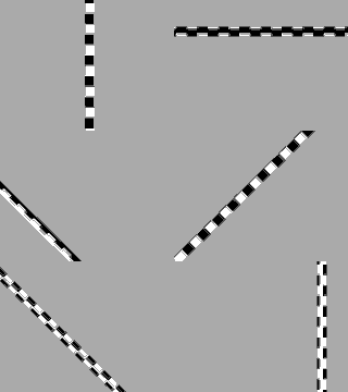
The visual stimuli are the familiar ones from retinotopy which are CW and CCW rotating 90 degree wedges and expanding and contracting rings. But, typically we also run bars stimuli in which a bar sweeps across the visual field in 8 different directions (its important that they sweep both forwards and backwards so that receptive field size and hemodynamic response width are not confounded. Also, we typically run the bars in a pseudo-random order but keep the same order fixed across repeated scans and average all of the data together). Another important point is that it is useful to turn off the stimulus (go to gray) for a cycle every now and then. This probes for very large receptive fields which may not be modulated by stimuli that move within the receptive field. The bars stimuli look something like this (note that the subject typically is fixating in the center on a fixation cross - not depicted - while doing a straight-forward fixation task):

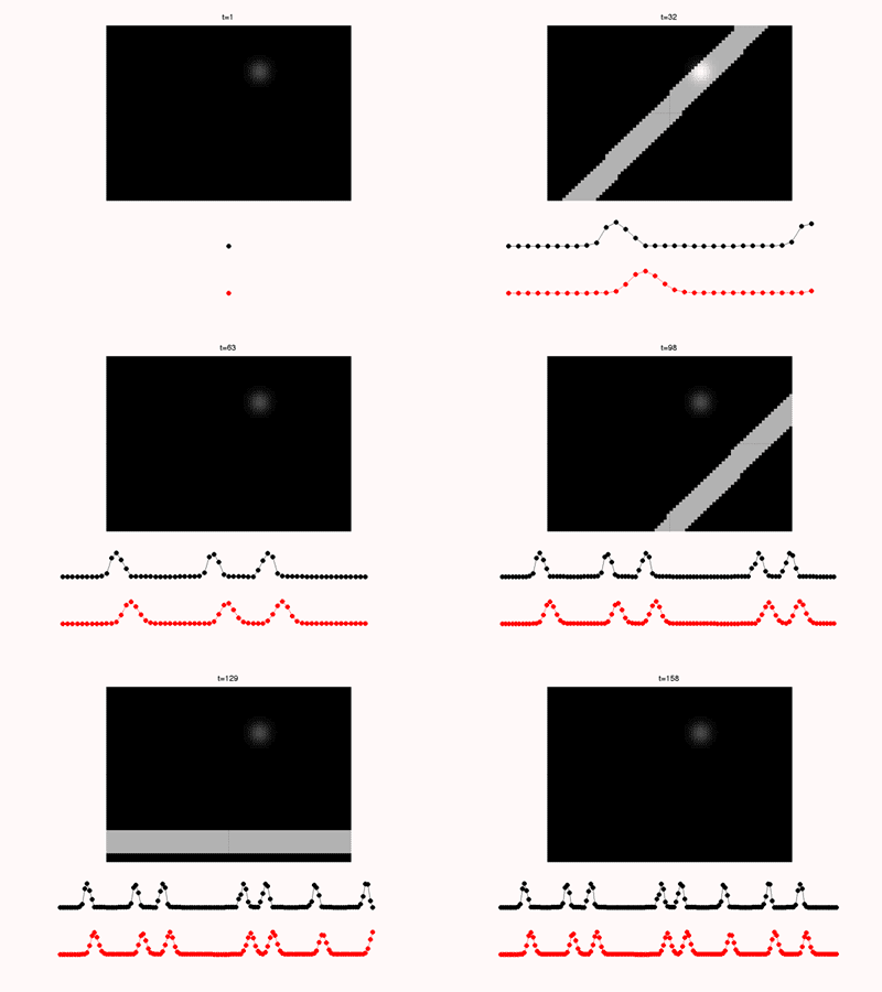
The pRF analysis is basically very simple. We hypothesize that each voxel has a gaussian shaped receptive field (the combined receptive field of the population of neurons which contribute to the response of the voxel). We then want to fit the parameters of this gaussian (x, y and standard deviation) such that the predicted response of the receptive field to the stimuli we presented best matches the actual measured time series. We make predicted responses, like the following:

What you see in the above is a small receptive field in the top right with the stimulus running over it in different directions. The black trace below is the time-point by time-point multiplication of the stimulus and the receptive field summed over all of space (it is the predicted response of the receptive field). That gets convolved with a hemodynamic response function to make the predicted BOLD response in red.

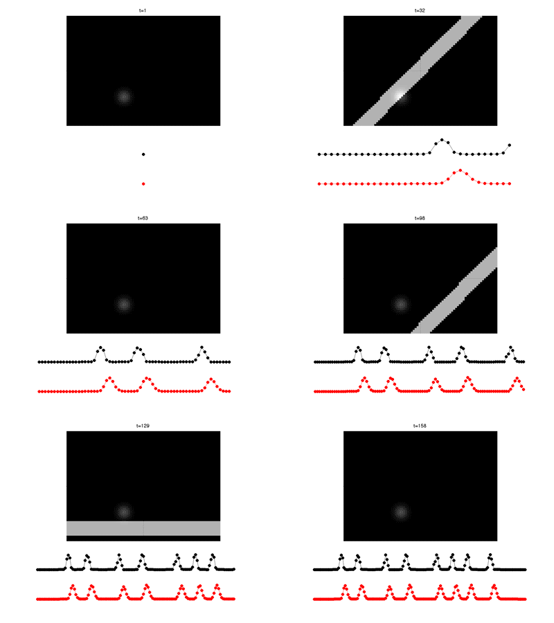
If you move the receptive field to a different location, it predicts a different time series:

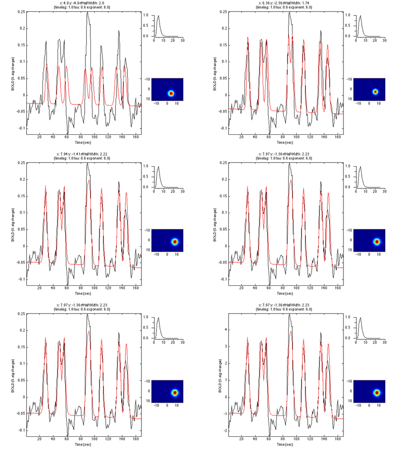
So, to fit a voxels response we change the position and standard deviation of the receptive field until the predicted response (red) best matches (in a least-squares sense) the actual time series for the voxel (note the lag in the BOLD response compared to the black trace).

Here is an example of a fit as it proceeds to change the receptive field position and size to best match the predicted time series (red) to the measured time series for the voxel (black):

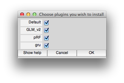
We start by doing a quick retinotopy analysis. This will be used as a reference. We will be using the pRF and GLM_v2 plugins (GLM_V2 provides some better user interface items). Make sure these are installed by doing:

>> mlrPlugin

and selecting from the dialog GLM_V2 and pRF. Note that if you have a mrLoadRet going already, you will need to restart it to have these settings take effect.

Now, go ahead and start mrTools by cd'ing into the experiment directory and running:

>> mrLoadRet([])

The scans are all labelled and you should be able to do this analysis w/out looking at the cheat sheet below. Note that the best shift used for these scans was -2. So, go ahead and average together appropriate scans with the correct shift and flip and then run the correlation analysis!

Cheat sheet

Really can't figure it out? Hmm. Consider doing the retinotopy tutorial again. In brief, here are the steps you need to accomplish.

(1) Check what scan is what. I like to do this from the command line by typing groupInfo('Raw') - you can also go to Edit/Group/Info. Note that typically we would need to run motionComp on these scans but for the tutorial sake this has already been done. GroupInfo will show you that Scan 1 and 5 were CCW, Scan 2 and 6 were CW and Scan 3 and 4 were expanding and contracting rings, respectively.

(2) Average together wedge scans. You need to do this with the correct shift and reversing. For the wedge scans, go to the Analysis/Averages menu item. Now unclick “include in average” and press the “copy” button - this removes all scans from the average. Now click “include in average”, set the shift to -2 and click reverse. Go to the next scan (2). Click “include in average”, shift = -2, and make sure that reverse is unclicked. Goto scan 5, “include in average”, shift = -2, reverse=clicked. Finally scan 6 and “include in average”, shift = -2 and reverse=unclicked. Check your work in the dialog box and click OK. (Make sure that only scan 1,2,5 and 6 are included in the average)

(3) Average together expanding/contracting rings. Same deal as wedges, average scan 3 and 4, time reversing one of them and shifting by -2 both. Make sure that only scan 3 and 4 are included and that all other scans are not included in the average.

(4) Check your work. Switch to the Averages group (drop down menu on the top-left) and get scanInfo (⌘I) for the first scan. The “scanList” field should read [1 2 5 6], shiftList should be [-2 -2 -2 -2] and reverseList = [1 0 1 0]. Also, make sure that the scan has 160 frames total with 0 junk frames (totalJunkedFrames should show up with 8 indicating that 8 frames were junked in the averaging step). If any of these are not correct, delete the scan and try again. Check the same for the second scan. If everything is good, you should go to Edit/Group/Edit Group and prepend the word “wedges” to the description and “rings” to the other scan. This will help keep track of everything.

(5) Run correlation analysis Go to Analysis and run the correlation analysis. Make sure “(Re-)compute” is checked for both scans and #cycles reads 10.

(6) Examine retinotopy Switch the base to s017LeftOccLarget (the flat patch for the occipital cortex on the left) by going to the Base dropdown on the top left and select it (If for some reason it is not loaded, you could also go to File\Base Anatomy\load and load s017LeftOccLarget). Click on co in the Clipping overlays block and set its minimum to be 0.3 (to get rid of some of the voxels not actually driven by the stimulus).

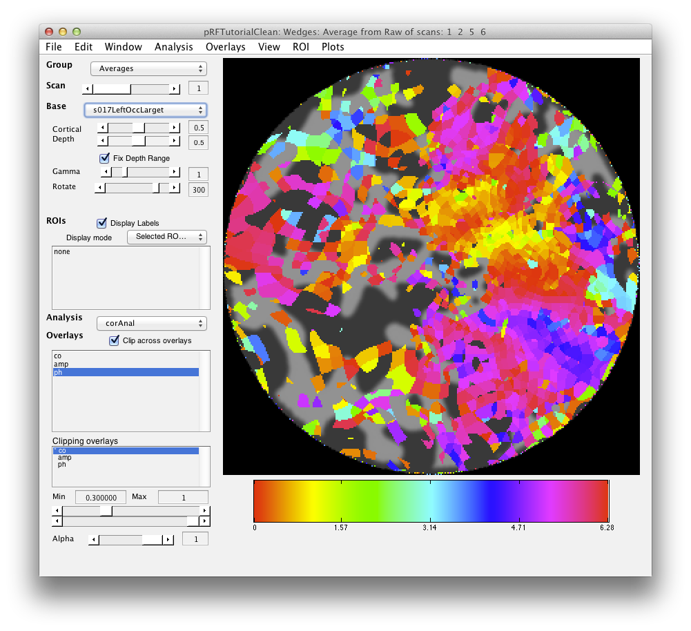
If all went well, your retinotopy should look something like this:

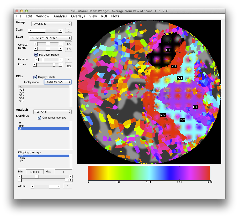
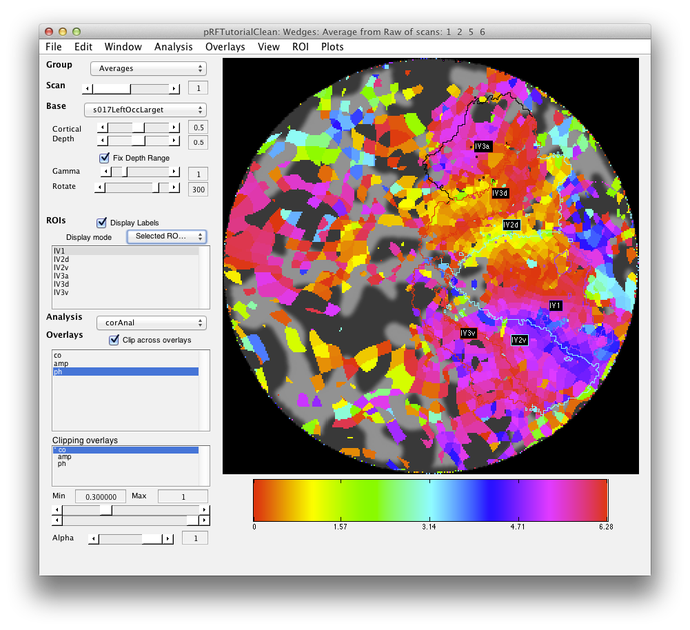
Now you should draw ROIs for V1, V2, V3 and V3a (hV4 is a bit broken up in this particular scan). Again you should be able to do this based on what you learned in the Retinotopy tutorial. For our version check the following:

Cheat sheet If you need help on drawing ROIs, check the Retinotopy tutorial here.

In the next steps you will average and concatenate scans for the pRF analysis. Note that this is different from what you do with the retinotopy analysis in which you shift and flip and do other tricks to account for the hemodynamic lag. For pRF analysis you are going to fit a model of the response which has the hemodynamic response lag as part of it. So you don't want to adjust the timing of the scans at all. This is important. If your scan timing is not correct relative to the stimulus all bets are off. In particular, you do not want to shift or reverse scans in averages. The code does handle junkFrames appropriately, but we are going to turn those off too. Remember that if you remove frames then your model has to know you did this otherwise it will associate the wrong stimulus with the response. So, here goes, let's make averages of like scans without any messing with the scans.

1. Turn off junk frames in the Raw group: You do this by going to the Raw group (Select from the group dropdown on the top left) and selecting Edit/Group/Edit Group and then go through and set Junk frames to 0 for each scan. This should automatically set the numFrames to 168. Click ok.
2. Average together the CCW scans (note that you do not want to include CW and CCW scans together since they had very different stimuli with different responses). Go to averageTSeries, include scan 1 and scan 5. Make sure that shift is 0 and reverse in *not* clicked. Make the same type of averages for CW (scans 2 and 6), Expanding (scan 3), Contracting (scan 4) and Bars (scans 7-10). You should end up with 5 new scans in your averages groups. Note that for Expanding and Contracting you will only have one scan - that's ok. This is just so that you have all the scans averaged as needed in the Averages group.
3. Check your work. Go To the Averages group. You should have a total of 7 scans now. Check the Edit/Scan/Info (⌘I) on each one of the scans that you just made to make sure that they are the average of the correct scans and that they do not have shift or reverse set. Also they should have no totalJunkedFrames or junkFrames and have a total of 168 volumes.

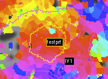
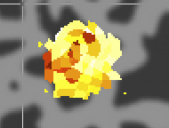
First make a very small ROI for testing. You can make the ROI anywhere, but inside V1 where the retinotopy produced good results would be a good place to start and for the sake of following through on the tutorial you may want to get a similar set of voxels as is shown below:

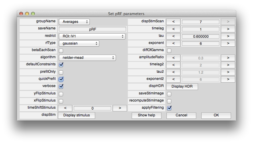
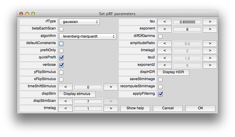
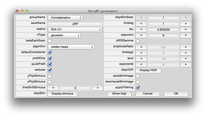
Now, from the Analysis menu select pRF. You should see a dialog box like this:

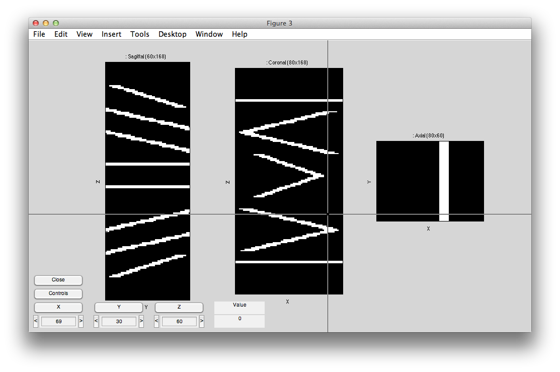
This sets the options for the pRF analysis. The help menu should give explanations for the options, so we will just cover a few things here that are essential to know. The pRF analysis needs to know the stimulus that was presented during the scan. The code retrieves this from the stim file. You can take a look at what it computes as the stimulus by clicking the Display stimulus button. For example, let's look at the stimulus for the 7th scan in Averages (the average of the bar stimulus scans). Set dispStimScan to 7 and click Display stimulus and you should see this (this may not work on a non-mac computer):

What you are looking at is the stimulus with different cuts through a volume with axis x and y (image dimensions) and t (time in Z dimension). So, if you click the Z button you should see what the stimulus looks like animated volume by volume. Note that for our calculations we consider the stimulus to be changing at the same rate as the data acquisition. That is, the stimulus changes position each volume. We are ignoring all of the sliding bars that you see in the stimulus shown above. A more sophisticated analysis might try to take into account every frame of the stimulus and use all of that to generate a pRF model, but here we just think of everything happening within the bar as contrast changes that stimulates a pRF and therefore the stimulus image is just showing areas in white where there was high image contrast and black where there was no image contrast. Click Close to close the stimulus view.

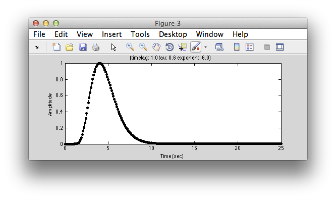
Next, lets take a look at the model hemodynamic response function. Click Display HDR:

You can change parameters of this function by changing the parameters (timelag, tau and exponent). It is simply a gamma function commonly used as a simple hemodynamic response function. If you want an hemodynamic response function that has a negative undershoot, click on diffOfGamma and display again. Usually you don't need to adjust this function, but if you have different assumptions about what a “canonical” hemodynamic response function is you can change parameters to get what you want. Note that the basic fit uses this common hemodynamic function shape and convolves it with the model response time series, you can also fit a hemodynamic function at the same time as fitting the receptive field. This is set by changing the rfType to “gaussian-hdr”. But, for now, let's stick with the basics. We'll get back to more advanced fitting in a little bit.

So, now let's run it. Make sure that “restrict” has the ROI you just created (otherwise it may take a very long time to compute - if you make a mistake and it is running too long, your only option is to hit ctrl-C in the command window, which will crash you out to the debugger, but won't have any other bad side effects). Click OK. Then select Scan 7 (the bars stimuli scan) from the dialog that pops up. At this point you may get a pop-up with the following:

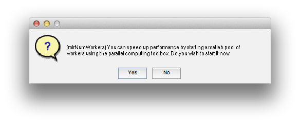
Basically, the algorithm work much faster if you use the parallel toolbox. By clicking Yes (this option may not be available if you do not have access to the parallel toolbox), it will start a number of threads each on a different processor of your machine. This speeds up things since on each processor you can be fitting a different voxel simultaneously. So, generally it is worth saying Yes to this dialog. Note that there appears to be some issue as of this writing (6/18/2013, Mac OS 10.8) with java and the parallel toolbox (the program will crash in matlabpool) that can be fixed by a patch.

It should now be fitting the time series. This can take some time depending on how big the ROI is that you made. You can check the progress in the matlab window.

When processing is finished, there should be 4 new overlays loaded (r2, polarAngle, eccentricity and rfHalfWidth). Switch to scan 7 and you should see an r2 map that looks something like this (note that if you click on a voxel within an ROI you may get a different plot - summary of the whole ROI - so either Hide all the ROIs (menu at left) or click on a voxel outside the ROI):

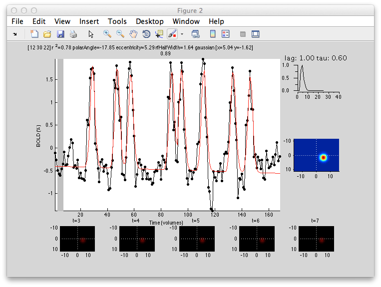
This shows the amount of variance accounted for by the model fit. You can examine the fit by interrogating voxels with the pRFPlot interrogator. To do so, make sure the interrogators are running (Plots/Interrogate Overlay) and make sure that the interrogator pRFPlot is selected in the bottom left of the screen. You may want to make sure that you hide your ROI viewing since clicking on a voxel within the ROI will bring up a different display which shows the fits of all the voxels as explained below. Now go click on a voxel. For example, if you click on the voxel [12 30 22] you should see the following:

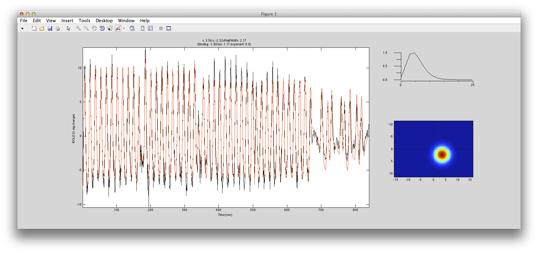
What you are looking at is the data in black with the model fit in red. The top right shows the model hemodynamic response function used (which should be the same for all voxels since we did not fit its parameters for this fit). Below that on the blue background is a display of the fitted RF. It appears on the right side of the screen which is a good sanity check since this is the left visual cortex. If you drag your mouse over the time series the gray bar should move. The gray bar is simply depicting the time window being displayed in the black/red images below. What those images are showing is the stimulus at that time (gray bar) with respect to the receptive field for that voxel (red).

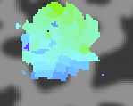
Now let's go back and look at the various other overlays. If you click on the polarAngle overlay you should see the following:

Note that you see a nice gradation as receptive fields are going from the lower right visual quadrant in green to the upper right visual quadrant in blue - just as is expected for the retinotopic ogranization of V1. You should click on individual voxels in green and in blue and be able to see in the interrogator window that the receptive fields are moving as expected. For example here is one from the green region which is more dorsal in V1 and thus responds to the lower visual field:

And here is one from the blue area which is more ventral and thus responds to the upper visual field:

Next click on the eccentricity overlay and you should see the following:

Again a nice gradation as expected from retinotopy. Lighter colors are more eccentric. If you click on voxels at various positions you should see the eccentricity of the RFs.

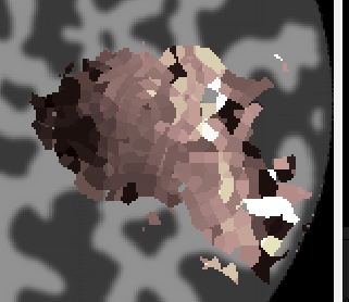
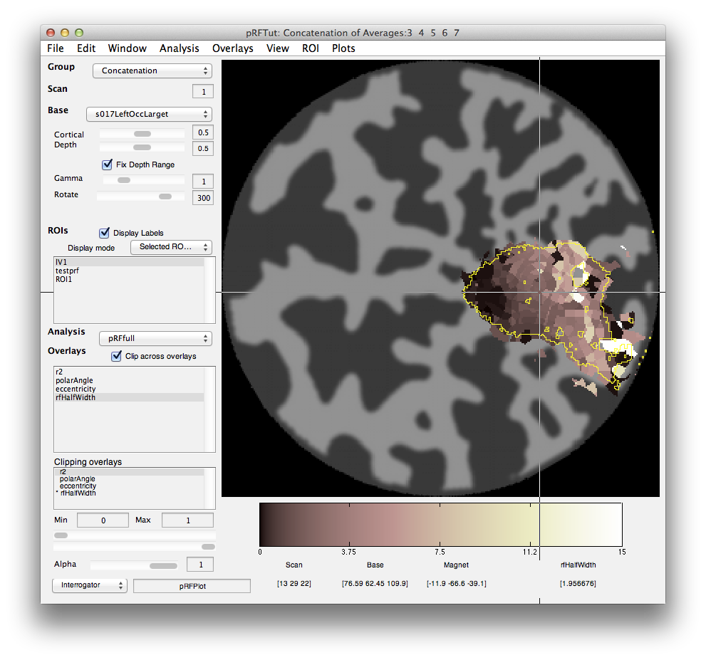
Finally, we can look at the rfHalfWidth. This is the size of the RF and is actually the std of the gaussian used to fit the receptive field. The map should look something like this:

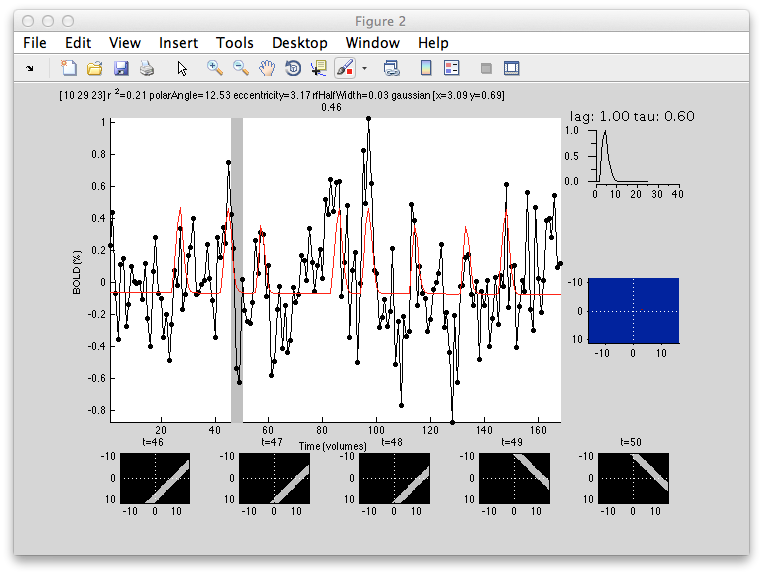
Its a bit noisier in the sense that there isn't as clear a gradation as for eccentricity, but if you squint there is a tendency for RFs that are bigger (lighter colored) to be more eccentric as expected from the known physiology. Note that there are some voxels that are black suggesting very small RFs. These are likely not real but one failure mode of the algorithm. Clicking on one of them (e.g. [10 29 23]) you can see what happened:

What happened is that the algorithm found that it could make the RF really really small and then account for a few time points in the time series (the red spikes you see). Basically what is going on is that for a tiny RF the response are very infrequent and so the algorithm can fit noisy single points in the data. Note that the variance accounted for by this fit is not as good as other voxels, so you can go set the Clipping Overlay r2 to have a minimum of 0.4 (make sure to have “Clip across overlays” checked, then click on the r2 in the Clipping overlays and set the min field), then you will see that all these black voxels are thresholded out:

Next we will try and refit the population RF using different options for the fitting parameters to better understand what is going on.

We will explore how to set constraints on the search. For example, the voxels with rfHalfWidth very small are unlikely to be real, so it would be nice to set a constraint on the algorithm to avoid it finding such a small RF.

To do this you can recompute the fits for specific voxels - in particular, choose a voxel that came up black in the pRF analysis rfHalfWidth map. What you need to do is make sure that input focus is on the mrLoadRet window (click on the title bar for instance). Now using the interrogator function, you should click on a voxel while holding the shift key down. (Note that this may not work on a non-Apple machine - if clicking on an individual voxel while shift is held down does not work, then just re-run the whole pRF analysis from the Analysis menu).

Make sure you keep the shift key down until you see the pRF options dialog box come up:

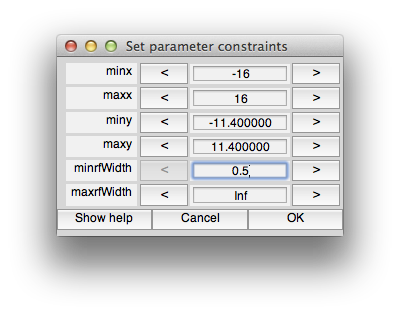
We can now set the constraints so that we don't allow fits with tiny receptive fields. To do this, we have to use the levenberg-marquardt algorithm instead of nelder-mead. This is because levenberg-marquardt is a non-linear minimization algorithm which takes constraints, but nelder-mead simplex method is an unconstrained search. Note that the default is to use nelder-mead because it doesn't seem to get stuck in local minimum as much as levenberg-marquardt. If you want to learn more about these algorithms books like “Numerical Recipes” are a standard reference. So, first we set the algorithm to levenberg-marquaredt. Next unclick “defaultConstraints”. Also click “quickPrefit” (more about that in a minute) and click “OK”. You should see the following constraints dialog come up.

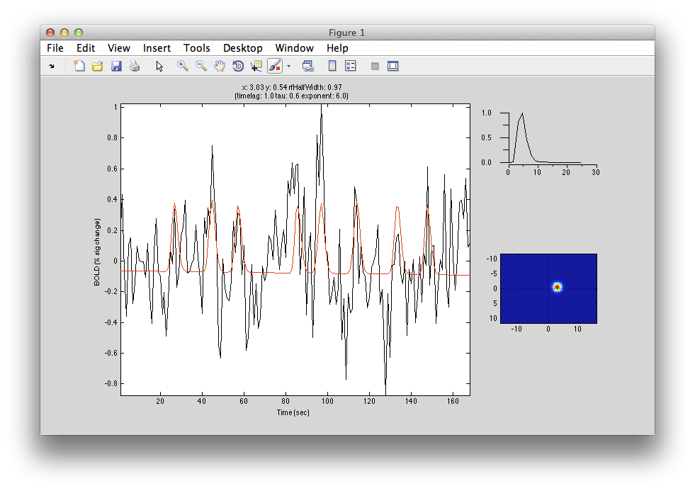
You can set constraints on any of the parameters, but for this case, let's just set the minrfWidth to 0.5 to keep from fitting a very small RF. Set that and click OK. After a minute you should see a window appear in which you can see the progress of the fitting algorithm (it should up-date from time to time with the RF moving around and the red model responses changing).

In this case, it settled on an RF slightly larger than the minimum (0.76) and still seems to have got the right location for the voxel (compare the x,y position with neighboring voxels in the map).

You may want to refit a few voxels and see how changing the constraints in various ways changes the fit that you get.

When doing nonlinear fits, the starting point of the algorithm often has a large impact on the optimal fit achieved. For example, if the initial estimate of the RF that you give the algorithm is very far away from ideal, the algorithm can get lost in the error space and stuck in a local minimum with parameters far from the global optimal. If you could tell the algorithm where to start - like that you should start in the contralateral visual field for instance, you could do better.

The way we deal with this problem is by computing a grid of model receptive fields at many different locations in the visual field with many different receptive field sizes. We then do a quick test - what we call “prefit” - to see which of these model responses is most highly correlated with the actual voxels responses. By choosing that RFs parameters as the starting point we could do a better fit.

But, how many model receptive fields to calculate? The more you calculate the longer the algorithm takes, but the better the starting estimate. So, there are a few options that you can play with here. Shift-click on a voxel to bring up the pRF parameters dialog box. quickPrefit only computes a small number of model responses. This is useful for testing things out quickly, but the problem is that you may not have sampled the space of RFs very well and so the algorithm later will get stuck in a local minimum. We note that this is particularly true with lavenberg-marquardt which seems to not move very far from the initial starting point. This is why we default to using the nelder-mead even though it cannot do constrained searches.

The other option to note is the “prefitOnly” option. What this does is compute the best RF just based on the prefit (no nonlinear search). It just matches the best model response with the voxel response and reports that as the fit. It is very quick and dirty and can give a pretty good idea of whether things are working or not, but the results will be quantized to only the RF locations and sizes that were computed.

Up to now we have been using a “canonical” hemodynamic response function. In some cases you may want to relax this assumption and actually try to fit the hemodynamic response. Note that when you do this there are more parameters in the model and lots of opportunities to get stuck in local minimum, so the fit gets harder to do. Nonetheless we can try to estimate the hemodynamic response function at the same time. Shift-click on a voxel with very high r2 like [10 31 20]. Now, in the options dialog box, change the rfModel to “gaussian-hdr”. Keep everything else with the default values - in particular, probably best not to do a quickfit since we need good starting parameters. You should see a window like this:

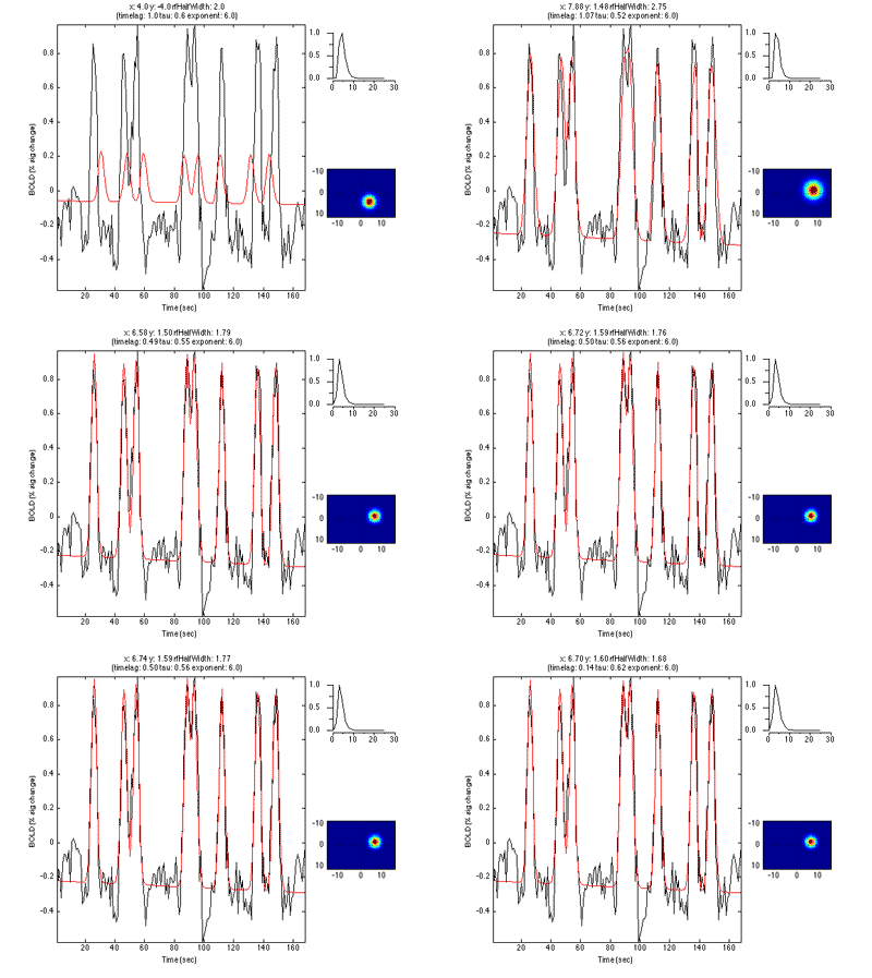
You can watch as the algorithm adjusts both the RF location and the shape of the hemodynamic response function to find the best fit. Here is in example of it doing the fit with the hemodynamic response:

Ok. Now we are ready to try a bigger ROI for a more real test. To do this, we are going to now concatenate all of our various stimulus types together so that we can use all of the data that we have.

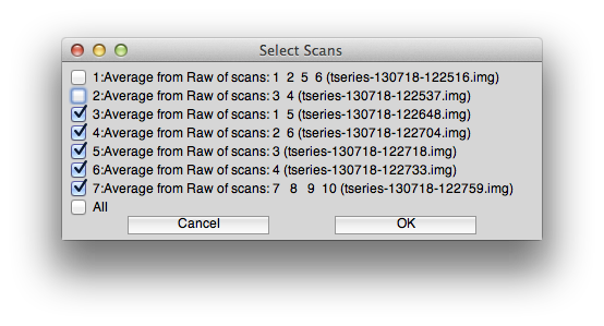
So, go to Analysis/Concatenate Time Series and concatenate scans 3-7 (make sure not to concatenate the scans 1 and 2 which were the ones used to make the standard retinotopy and have the response time series shifted and reversed). You can use the standard options for filtering and the like on the concatenate dialog box. The scans you select should look like this:

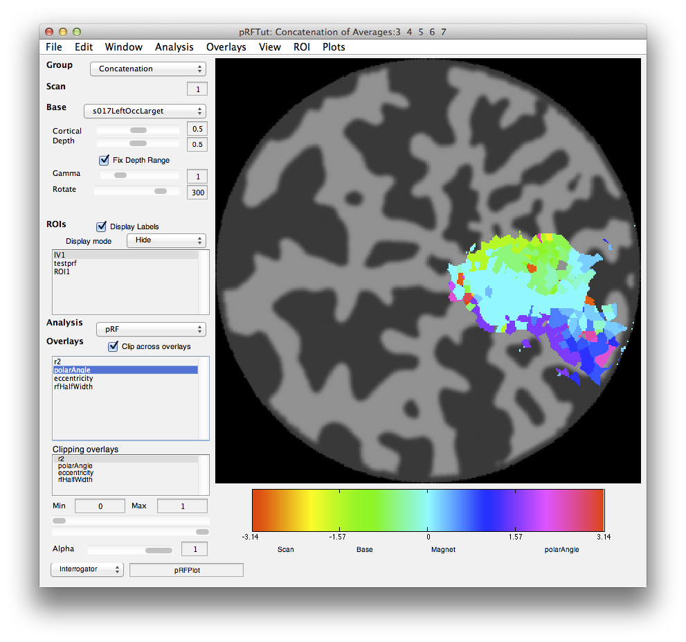
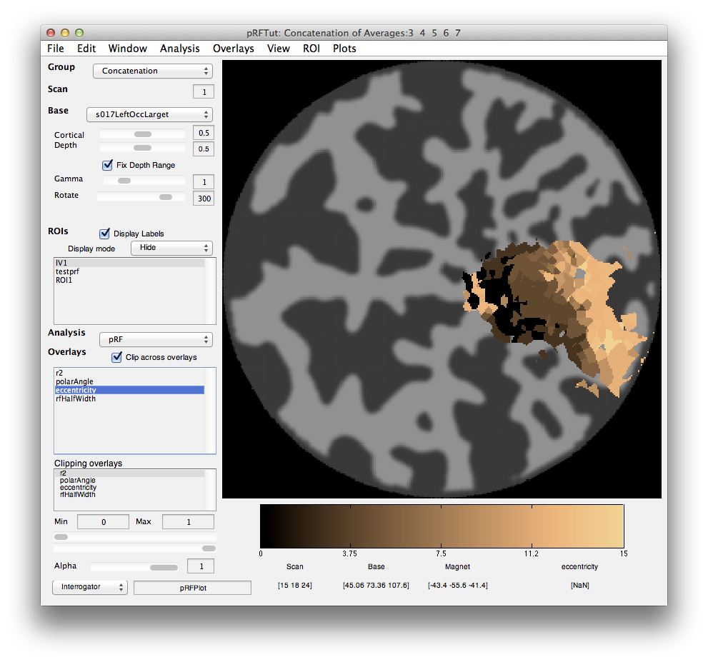
Now, switch to the Concatenation group and select Analysis/pRF. Let's do a quick and dirty prefit only to see what things look like. Click “prefitOnly” and “quickPrefit” and make sure that the restrict ROI selected is for your V1 ROI.

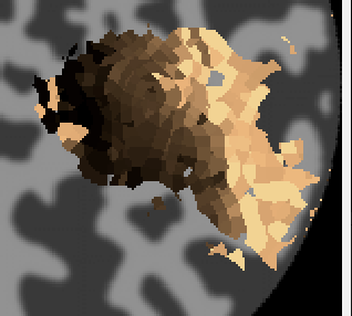
This may take some time to run. Works best if you are using the parallel toolbox and you have lots of free processors! After some time it should complete and you get a rough polarAngle map that should look something like this:

And the eccentricity map should look like this:

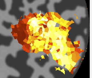
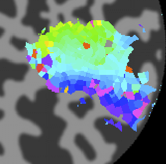
Looks reasonable! If you have the processing power and the time to wait, you can try a real fit. Just run pRF from the analysis menu again, but this time use all the default options and click OK. Wait some time and you should get maps that look like the following. Things look generally smoother and cleaner with the exception of a few voxels here and there that are not fit well:

r2 map:

Polar angle:

Eccentricity:

and rfHalfWidth:

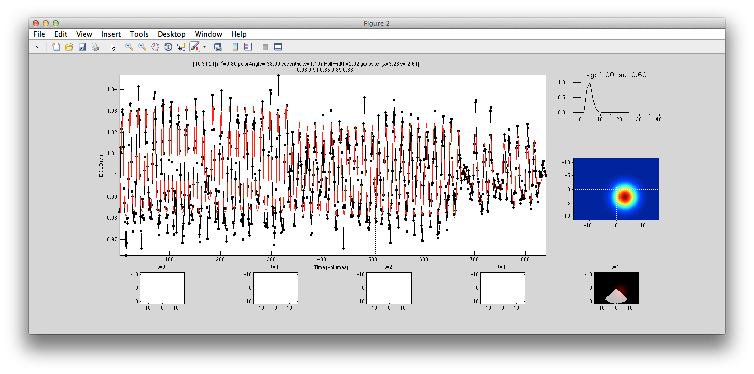
If you click on a voxel (say [10 31 21] that has been well fit with the interrogator, then you should see that it is using the full time course across many experiments and doing a pretty good job of fitting all the data (compare red model curve to data in black). Notice that the overall r2 for this voxel is accounting for 80% of the variance. In individual scans within the cocnat (second row of title), we see that it is account from 85% to 93%.

Finally, if you have the V1 ROI showing and click a voxel within the ROI:

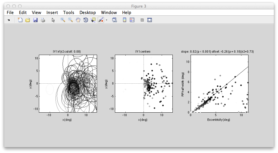
You can examine all the RFs within the ROI together. You should see a figure like the following:

Left shows all the RFs drawn on to the visual field - they all are in the contralateral (right) visual field and look like they do a reasonably good job of tiling that space. The plot of RF half width (std of gaussian receptive field) against eccentricity shows a nice linear relationship which is also what we expect in V1.

-jg.