Table of Contents
Classification tutorial overview
This tutorial explains classification analysis with fMRI data using mrTools. Classification analysis can be used to examine distributed patterns of activity - often subtle responses that are hard to examine with other methods. For example, the responses to different orientations which might be distributed across the cortex (see: Freeman et al and Sasaki et al for how they are distributed). Kamitani and Tong showed that you could use classification techniques to read-out the orientation representation. That is, they build classifiers on a subset of data collected as subjects viewed gratings of different orientations and then tested that classifier with a left-out set of data. They were able to show that they could correctly determine what stimulus orientation subjects had been looking at, just by looking at their fMRI measured brain activity. Here we will go through what you need to know to do these types of analysis. The tutorial has one section on basics about classification (not necessarily about fMRI) and another section which uses actual fMRI to do a very simple classification analysis (was a stimulus presented above or below the fixation point?).
To run the tutorial you will need to have some matlab files, that you get by downloading the following file classification.tar.gz. After downloading, you should be able to either double-click the file to make it into a directory, or from the command line do:
gunzip classification.tar.gz
tar xfv classification.tar
And then add it to your path in matlab.
>> addpath(genpath('~/directoryWhereYouDownloaded/classification'));
This is all you need to do for the first part of the tutorial.
If you want to try the second part of the tutorial where you test some of the ideas on real data, then you can download the datahere. Its a big file, so it may take some time to download (approximately 430MB).
The files are provided as a tar/zip file. In Mac OS X you should be able to just click to open the files in the Finder. Otherwise, you can go to a terminal and do:
gunzip classificationTutorial.tar.gz
tar xvf classificationTutorial.tar
You should familiarize yourself with the basics of data analysis in mrTools by doing the retinotopy tutorial and the event related tutorial before going through this tutorial.
Some documentation for these functions can be found here.
Classification Basics
Mean classifier
In this first part, we are just going to play around with different classifiers to see how they perform on data to get a feel for the strengths and weaknesses of different methods.
We begin by creating a set of test data. What we want is two sets of data from two different classes. For classification in the context of fMRI data you can think of these as responses generated from two different kinds of stimuli or different kinds of tasks etc. Each dimension is the response (usually the average over some period of time) of a different voxel. For the test data we will create and use data with only two dimensions so that it is easy to visualize and understand what is going on - meaning that it is like using fMRI data from only two voxels. Conceptually, everything should generalize to multiple voxels. But, beware of the "curse of dimensionality" in which adding dimensions increases the volume of the space that one has to search for solutions in - this can occasionally cause problems.
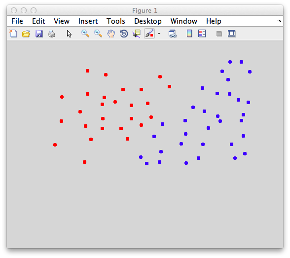
Ok. So let's create the simplest case for a classification. Two data sets that are separated from each other and should therefore be easily classifiable. We will define the points ourselves by using the program classifyTest:
[x1 x2] = classifyTest('type=none');
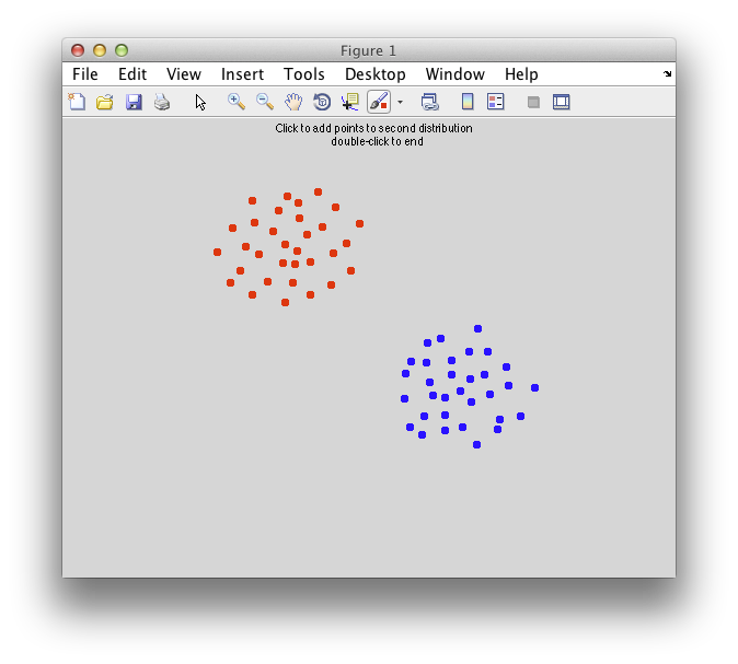
On the graph, click 20 or 30 points roughly in a circle in one location and then double-click the last point. Then make the second set of 20 or 30 points in a location slightly removed. It should look something like this:
Ok. Now in x1 and x2 we should have the coordinates of all the points that we made. You can take a look at them:
>> x1

x1 =

        -0.673963133640553          0.87280701754386
        -0.763824884792627          0.68859649122807
        ...
>> x2

x2 =

         0.383640552995392         0.013157894736842
         0.197004608294931        -0.171052631578947
         ...
Only the first few points have been shown. If you want to use nearly exactly the same data as is shown in this tutorial. Copy and paste the lines in the following to your matlab buffer:
To define some terminology here. We have two classes (red and blue points now named x1 and x2, respectively). Again, classes can be response to different kinds of stimuli (horizontal vs vertical orientation) or different kinds of tasks (adding vs subtracting numbers), anything you like. Each row is an “instance” of a response to each class. It has two columns, which would be the responses of voxel 1 and voxel 2 to that instance.
Linear classifiers are defined by the “projection line”. This is the line (and its a line even if you have more than two dimensions for your data) upon which you project all new instances. Projection means to drop a line from each instance (which is a point in the space) perpendicular to the projection line. The point where this intersects the projection line is called the projection of the point and is also the point that is closest to the instance on the projection line. It is easy to find the projection - you just take the dot product of the vector that defines the projection line and the instance.
Once you find the projection of each instance on to the projection line you compare it against a bias point if it is less than the bias point you are going to say the instance comes from the first class and if it is larger than the bias point it comes from the second class. That's all there is to a linear classifier. Just to repeat, you do the following:
- Get the projection of each new instance on to the projection vector by taking the dot product of the instance and the vector that defines the projection line
- Compare that to the bias point (note that the projection is always a scalar value)
But, how to define the projection line and the bias point. Let's start with the easiest of all classifiers. We will define the projection line as the line that intersects the means of the two class distributions. Let's see what that does. First let's get the mean of both distrubtions:
m1 = mean(x1)
m2 = mean(x2)
We now pass it into classifyTest to have classifyTest classify based on this projection line. Do the following:
classifyTest(x1,x2,'projectionLine',[m1;m2]);
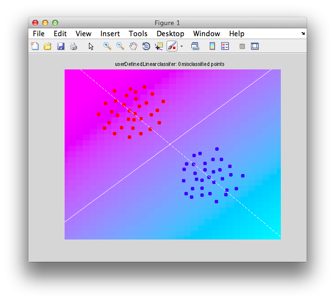
You should see a graph that looks like the following:
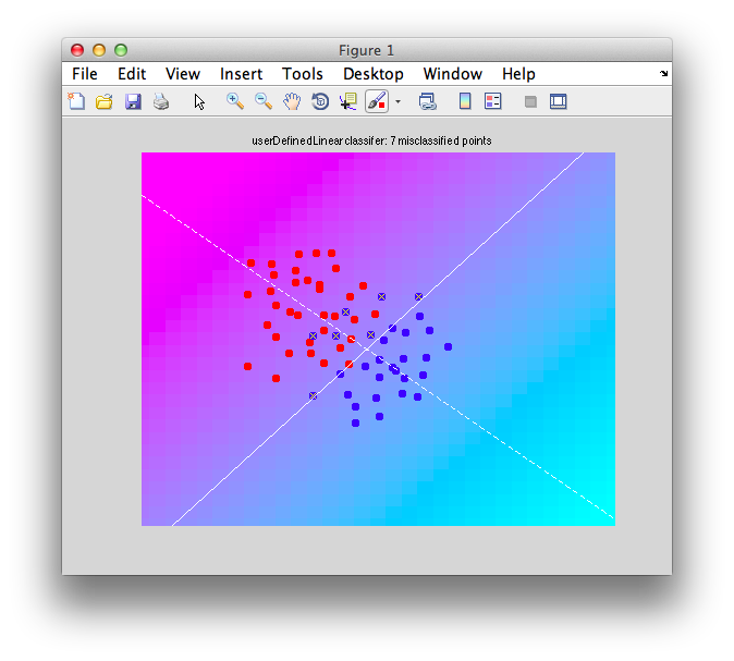
Note that there are two lines that are drawn. A white dashed line which is your projection line. Try to visualize what each point would look like if you drew a perpendicular from the white dashed line to each point and placed each point (instance) onto that projection line. There is a solid white line which is the decision boundary it is defined to be perpendicular to the projection line and is centered on the projection line at the bias point (which has been chosen for us as the point in between the two centers of the distribution that we passed in). Note that the decision boundary is in general an n-1 dimensional plane. That is, if we had k voxels instead of the 2 voxels of data in this case, the decision boundary would be a k-1 dimensional plane. The projection line would still be a line. The decision boundary you can think of as a wall that separates points into two different classes.
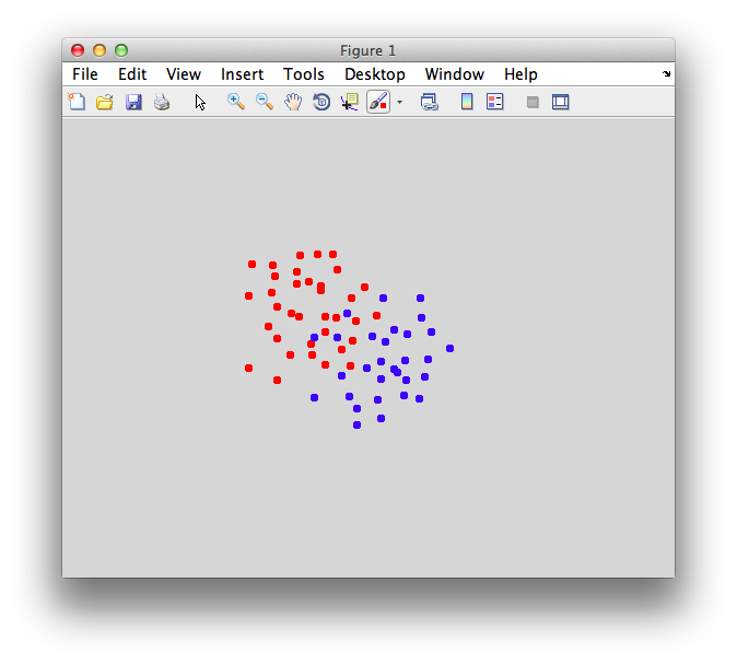
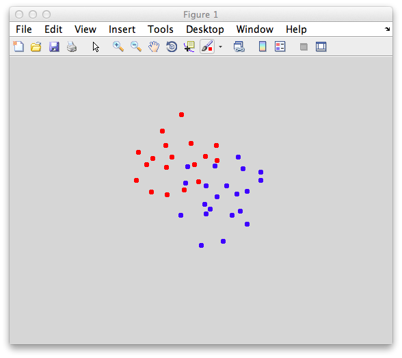
Ok. That was easy, but what happens if there are overlapped points? Let's make some points that are overlapped:
[x1 x2] = classifyTest('type=none');
You should make points that look overlapped like this:
Again get the means of the two classes to define a simple classifier that simply projects each point on to the line defined by the means:
m1 = mean(x1);
m2 = mean(x2);
classifyTest(x1,x2,'projectionLine',[m1;m2]);
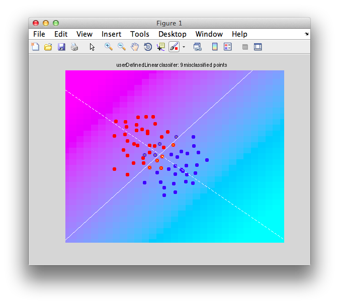
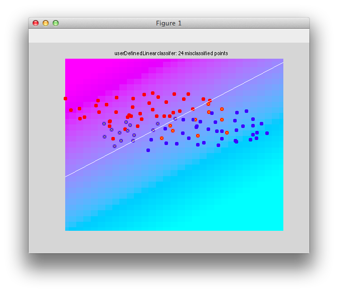
It should look like this:
Note that there are some misclassified points that are marked in x that end up on the wrong side of the decision boundary. Note that this is not a good way to test a classifier since we are testing with the same set of data that we built with - this can cause very serious problems of overfitting - more on that later and how to do cross-validation to avoid these problems.
Bias point
Remember that we said that the linear classifier is just a projection line and that we just use the dot product of the vector that defines that projection line and each instance and compare that to a bias point? Let's go through that step-by-step. We have been defining the classifier according to the projection line that goes through the two means of the distribution and that is what we pass into the function classifyTest. However, what does it mean the vector that defines the line? Well, this is actually meant to specify just the direction of that line which is defined as a vector w as follows:
w = m2-m1
Quite simple, huh? You can pass that into classifyTest to make sure that gives the expected results:
classifyTest(x1,x2,'w',w);
Now, let's talk about the bias point. How do we calculate that? The code has been setting it for you (that is, behind the scenes when you define the classifier weights, a calculation is being made for where the bias point is, and now we are going to compute that ourselves). Its worth understanding what the code does to define this bias point. So, lets just enter an arbitrary bias point that won't work. Like 0:
classifyTest(x1,x2,'w',w,'biasPoint',0);
You should see that the output has the decision boundary in the wrong place and so more instances get misclassified:
To find a better boundary, we can find out where each one of the instances in each distribution project on to the classifier line and then find the midpoint between these two distributions. So, to get the projection we simply take the dot product of the weight vector times each one of the instances;
for i = 1:size(x1,1)
  p1(i) = dot(w,x1(i,:));
end
Note that dot product is simply multiplying each dimension of each instance by the corresponding element of the weight vector and summing over that. That is why we call it a 'weight' vector. The larger the value in w, the more weight is given to the value of that dimension. So, just to be clear, for example dot product for the first instance is calculated as:
firstInstance = x1(1,:);
projection = sum(w(1)*firstInstance(1) + w(2)*firstInstance(2));
The value projection should give you the same value as p1(1). Now, on with computing the best bias point. Lets find the projection of the other class on to the projection line:
for i = 1:size(x2,1)
  p2(i) = dot(w,x2(i,:));
end
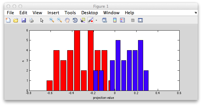
Ok. So let's look at the projection values for each class as distributions. Note that this is now one dimensional since it is the scalar values on the projection line. This is the point of the classifier - it turns the k-dimensional (in our case 2D) instances into a one dimensional scalar value which can best distinguish the two classes. Let's look at that:
  figure
  [n binX] = hist(p1);
  bar(binX,n,'FaceColor',[1 0 0]);
  hold on
  [n binX] = hist(p2);
  bar(binX,n,'FaceColor',[0 0 1]);
You should see something like this:
Notice that the distributions are pretty well separated. That's because the classifier is doing a good job of turning our 2 dimensional instances into one dimensional points (the projection onto the projection line) that best separates out the two classes.
Now, to best separate out the two classes, we just need to find a good boundary in this one dimensional space that separates out the two distributions. The center point between the mean of the two distributions will do (assuming equal variance of the red and blue distributions):
mp1 = mean(p1);
mp2 = mean(p2);
biasPoint = (mp2+mp1)/2;
You can draw that biasPoint on to the distributions to see what it looks like:
vline(biasPoint);
You should see that with this bias point you only misclassify a few of the points. To see it in the original space, we can set it in classifyTest:
classifyTest(x1,x2,'w',w,'biasPoint',biasPoint);
Note, now you know all it takes to build and test a linear classifier. To build you need to specify a projection vector (i.e. a weight vector) and the bias point. To test, you take the dot product of a new instance (not in the build set) and the weight vector and compare against the bias point. So, you can classify any instance you want by hand. For example, say the fourth instance in the first class:
testInstance = x1(4,:);
dot(w,testInstance) < biasPoint
This should return true, saying the point is in the first class (unless it happens to be a point that is misclassified). Take another point from the second class and it should return false (again, unless it is misclassified):
testInstance = x2(7,:);
dot(w,testInstance) < biasPoint
Check all the values in p1 and p2:
p1 < biasPoint
p2 > biasPoint
These should be mostly 1 - correct classification (note again that this is not a real test since we are building and testing with the same data set). But, anyway, if you want to compute the percent correct, you would do:
(sum(p1 < biasPoint) + sum(p2 > biasPoint))/(length(p1)+length(p2))
Naive-bayes classifier
So, we've been working with a very simple classifier (projection line in the direction between the two means). When does this fail? Well, for one thing it doesn't take into account different variance in different dimensions of the data. One voxel may have the same mean difference between different classes but be so noisy as to provide no reliable difference compared to a voxel that has the same mean difference but very little variance. We can set up this situation by making up some data using classifyTest:
[x1 x2] = classifyTest('type=none');
Something like this:
Copy and paste the data below if you want to use the exact same data as in the tutorial instead of defining your own points:
Now, let's try the mean classifier:
mx1 = mean(x1);
mx2 = mean(x2);
w = mx2-mx1;
classifyTest(x1,x2,'w',w);
This classifier basically weights both dimensions equally even though clearly there is more variability in the dimension on the abscissa:
So, what's the problem with this solution? Well, if you were to do it by eye, you would probably want the decision boundary to be more horizontal - that is, you would want to ignore the differences in the dimension on the abscissa which have high variability, but weight more the differences in the ordinate which has much less variability. Another way to put that is that you want to weight each dimension by the inverse of its variability. The higher the variability in the dimension the less you want to weigh it. So, let's just do that. First let's calculate the standard deviation each dimension (we do this pooling across both classes):
s = std([x1 ; x2])
You should see that s is larger for the first dimension than the second. That is there is more noise on the first dimension (think voxel) than the second dimension (voxel). So, you should adjust the weights accordingly. That is, make the weight on the first dimension smaller because its standard deviation is larger. To do so, multiply each dimension, by the inverse of the standard deviation.
w = w * 1./s;
Now, let's see if that does a better job:
classifyTest(x1,x2,'w',w);
Better. The decision boundary has now rotated slightly more horizontal and gets the fact that there is less variability in the dimension on the ordinate than the dimension on the abscissa.
This solution which assumes that dimensions do not covary is sometimes called a Naive-bayes classifier. Personally, that name doesn't do much for me. But they say that the “naive” part comes from naive thinking that dimensions don't covary (more in the next section about this) and the Bayes becuase this is a Bayes optimal solution for gaussian distributions with equal variances and no covariance.
Fisher Linear Discriminant
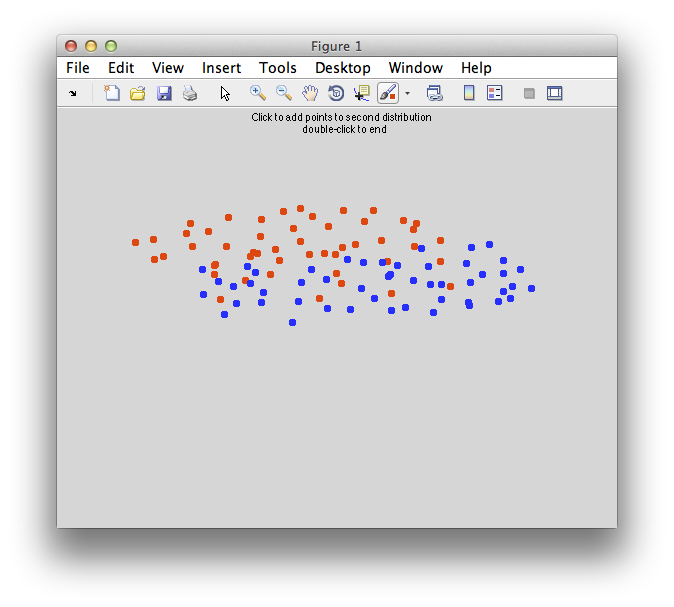
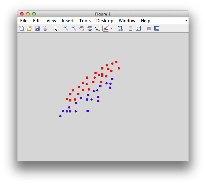
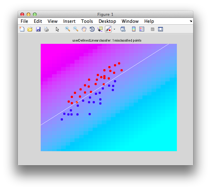
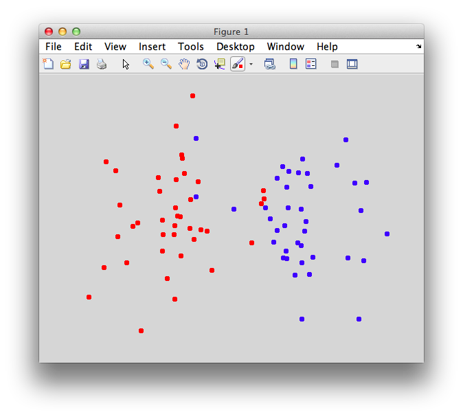
So, incorporating the inverse of the standard deviation is a good idea. But, is this enough? Consider the following case in which there is covariance between the response of the two dimensions. That is the higher the response is in one dimension, the higher the response in the other dimension. This can often happen with fMRI data in which neighboring voxels responses covary:
You may want to copy and paste this data set and try it out yourself:
Let's try the tricks we have in our playbook for dealing with this. First the mean classifier:
m1 = mean(x1);
m2 = mean(x2);
w = m2-m1;
classifyTest(x1,x2,'w',w);
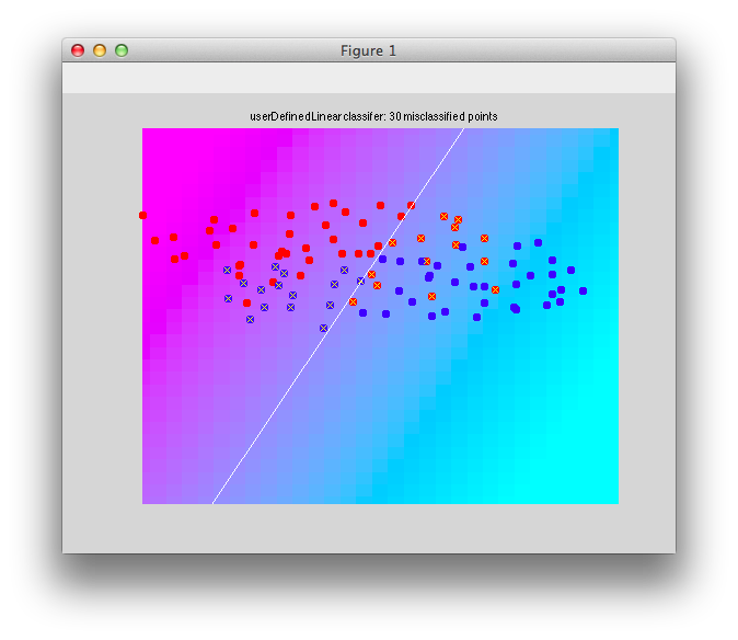
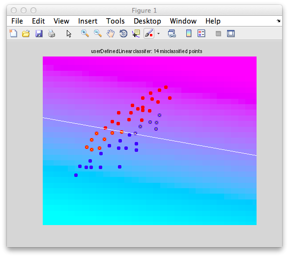
And, we get this:
Terrible! What happened? Well, look at the distribution on the abscissa they have a slight difference with the blue to the left of the red and on the ordinate the red is slightly higher than the blue, so the border is correct for the means, but its missing the dead obvious - it should be tilted up and to the right instead of down and to the left.
Ok. So let's go with trick two in our playbook. Let's scale by the inverse of the variances:
s = std([x1;x2]);
w = w.*(1./s);
classifyTest(x1,x2,'w',w);
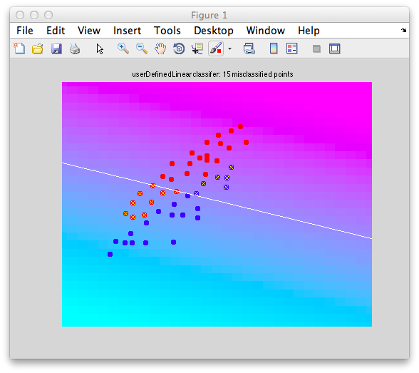
And we get:
And that helped us, not one bit. Why? Well the variability in each dimension is about the same so weighting by the variability doesn't change a thing.
So, that gets us to thinking about the defining characteristic here - that the responses in the two dimensions covary. We need to use that fact to define the decision boundary. To do so, let's start by calculating the covariance:
c = cov([x1;x2])
If you take a look at c:
c =
         0.126125531914894          0.11893085106383
          0.11893085106383         0.172812588652482
Note that the values on the diagonal are just the variances in each of the dimensions (compare to what var([x1;x2]) gives you. And the value in the top right (symmetrical with bottom left) is the covariance between the two dimensions. So, how should we use this? Well, before we scaled by the inverse of the variances. Doing essentially the same with the covariance matrix here just generalizes that. So, let's scale the mean classifier with the inverse of this covariance matrix:
w = inv(c) * (m2-m1)';
And, Bam! That does the trick:
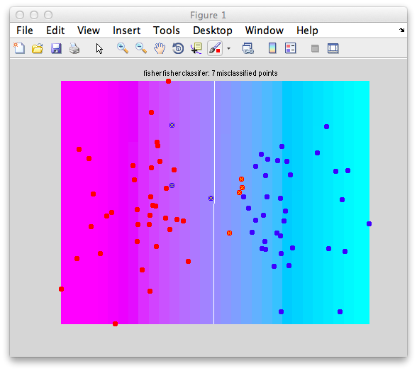
classifyTest(x1,x2,'w',w);
Why does this work? Well because it takes into account the means, properly weights it by the inverse of the variances (remember that the variances are on the diagonal of the covariance matrix and it takes into account the covariance of the two dimensions. Turns out this formulation - scaling the mean classifier by the inverse of the covariance matrix - is the right thing to do (in a Bayesian optimal kinda way) to solve any classification problem in which the variables are gaussian distributed with equal variance. It has a name. It's called the Fisher Linear Discriminant (remember that, cause it's a great solution!).
Support vector machine
So, Fisher Linear Discriminant works ideally for identically distributed gaussian data - but are there times when it fails? You, bet! When the distributions are not gaussian. We'll get into one way that the fail (and actually a way that all linear classification schemes fail), but first let's talk about support vector machines.
An alternative to Fisher Linear Discriminant for finding a good decision boundary starts from consideration of what makes a good decision boundary. Well, one might think, a good decision boundary is one such that the distance between that boundary and the points of each of the two classes is maximized. For support vector machines, this is called “maximizing the margin” - the margin being the space around the decision boundary without any points from either distribution. So, what does that look like? Make two distributions like this:
And let's calculate the decision boundary that maximizes the margin with classifyTest:
classifyTest(x1,x2,'type=svm');
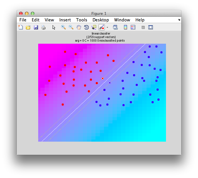
And we get this:
If you look at this there is a solid white line (the decision boundary) and the dotted lines neighboring define the margin - the largest distance from that boundary to any point in either distribution. The instances that are contacted by the margins are highlighted with a white border. These instances are called “support vectors” because they are the vectors (i.e. instances) that support the solution. If you changed those two points (like removed them), you would get a different solution to the problem - i.e. a different decision boundary that “maximizes the margin”. Indeed, you could remove any other instances from the distributions, the solution wouldn't change at all. It is only these support vectors that matter. Thus the name.
So, how did we calculate this decision boundary that maximized the margin? Well, you could think of it like this. We could try every orientation and position for the boundary calculate the margin for that decision boundary and then choose the decision boundary that had the largest margin. That would work, but would take a long long time. Instead, there is a clever math solution to this. It turns out you can compute the solution by converting the problem of maximizing the margin into a dual problem which if solved can be converted into the solution you want and then use a well known quadratic programming solution to that problem. So, the solution can be calculated very efficiently. The math is very clever - much too clever for me to explain, but there are a number of good sources if you are interested in learning more (Pattern Classification, Duda, Hart & Stork p. Chapter 5 ; A Tutorial on Support Vector Machines for Pattern Recognition, Christopher J.C. Burges, Data Mining and Knowledge Discovery 2, 121-167 (1998) and An introduction to kernel-Based learning algorithms, Muller, Mika Ratsch Tsuda and Scholkopf, IEEE Transactions on neural networks 12.2 (2001))
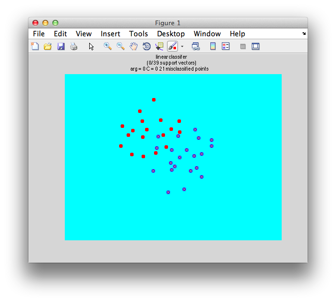
One thing that may be a bit mysterious, is, what if there is no margin in that the two distributions overlap, like (make some points like the following):
Well, there is a sort of fudge factor parameter C. The larger that C is the more tolerant the algorithm because. That is, if C is 0, then the solution will fail because it can't tolerate any instance being on the wrong side of the distribution. So, for example, if we set C to 0:
classifyTest(x1,x2,'type=svm','C=0');
We get this - total failure:
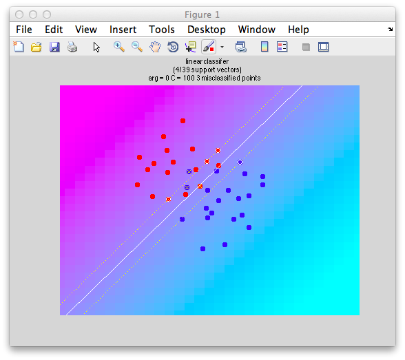
If we set C to a positive value, you get a reasonable boundary since it ignore the fact that some of the instances are on the wrong side:
classifyTest(x1,x2,'type=svm','C=100');
Note that it still computes “support vectors” as before, but it ignores the fact that there are other instances within the margin and even on the wrong side.
Play around with changing different C values to see the effect. How would you set this value in practice? Well, you could either just set it arbitrarily to some number or you could use cross-validation to find an optimal C value on some test set of data. In actually for high-dimensional data like those from fMRI experiments, it doesn't come into play very much. Why? The curse of dimensionality. It turns out that as you add many dimensions to data, the distance between any two arbitrary data points in the multidimensional space tends to be far away and in practice this means that there are decision boundaries that can be found in which points do not overlap - even if it seems like it in these simple cases with two dimensions (voxels) that would rarely happen.
Now, you should go back and try the svm solution on any of the data that we used before - for many it will end up giving you almost identical solutions as Fisher Linear Discriminant. So, why bother? Well, the real beauty of svm is that you can handle non-linear boundaries.
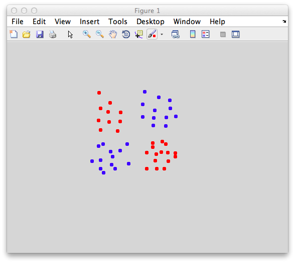
So, here is a problem that busts any linear classifier including Fisher - the dreaded xor. Xor (exclusive or) is a really, really simple function - just return if one of the inputs is high, but not both. In graphical form, it looks like the following:
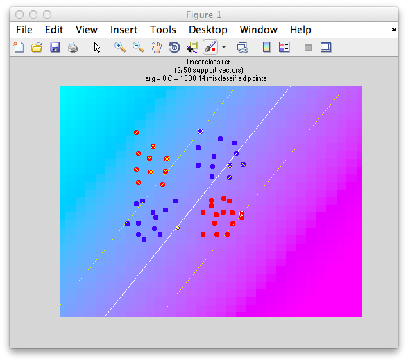
This is an xor problem because you have to only accept points into one category (red) if it has a high value (like a 1 for the logical case) in one dimension and a low value (0) in the other dimension, but not if it has two high values (1 and 1) or two low values (0 and 0). An svm classifier fails miserably:
classifyTest(x1,x2,'type=svm')
Why does it fail? Well, basically no matter how you split it, you can't cut a straight line through these points to get everything right. Any linear classifier including Fisher Linear Discriminant will fail.
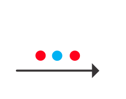
So, what to do? Well, we need a non-linear boundary of course. But, well, that's hard. So very clever people figured out a simpler solution - just add non-linear combinations of your dimensions to your data and then use the good old linear classifier in this new space to do classification. Huh, what? Well take a look at the following:
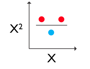
This is another version of the xor problem but in 1 dimension. There is no boundary that you can put between these points to correctly classify them all. But, if you just add a second dimension which is calculated as the square of the first dimension, you get a 2 dimensional problem which is now separable:
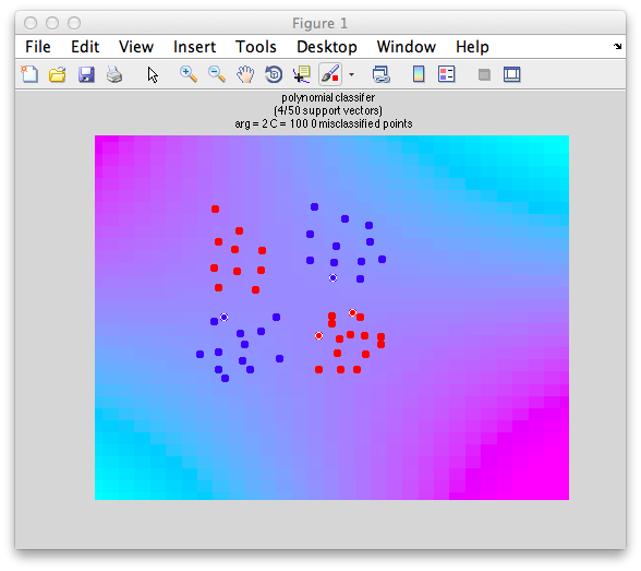
So, just adding a new dimension (calculated as a square of the first dimension) to your data allows you to use a basic linear classifier to beat the problem. So, we could just add new dimensions to our data by computing squares and so-forth, but then our data would get huge. It turns out for support vector machines (and this is a really nice property) the data only appear in dot products with each other and so instead of calculating non-linear new dimensions you can just transform the dot products and this is really quick and easy to do. So, here is a solution with svm in which we add a squared dimension by using this trick of squaring the dot products of the data:
classifyTest(x1,x2,'type=svm','kernelFun=polynomial','kernelArgs=2','C=1')
Note that we don't actually draw the boundaries for technical reasons, but you can see the cyan/magenta boundary fitting the data we made properly and that there are no points that are misclassified. And, here is the rub. Overfitting. With non-linear classifiers you can easily overfit data by getting boundaries that neatly follow the randomness of the data that you have and not generalize well to new data. Consider the following data:
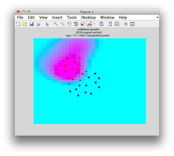
We can try a funky non-linear classification scheme (in this case instead of polynomial function we use a radial basis function - simply a gaussian function to transform into a new dimension):
classifyTest(x1,x2,'type=svm','kernelFun=radialbasis','kernelArgs=1')
And we get this:
Note the funky boundary evident - is this a good generalization of the data? Probably not. How does one avoid this. Two things. One, avoid non-linear classifiers unless you have a very good reason to believe that your data will need non-linear boundaries (like you know you have data with the xor problem). Second, use cross-validation.
Cross validation
There's not much to say about cross-validation except that you must must do it. Build the classifier on some data (build set) and set and test it on some left out data (test set). You can do this by splitting the data in halves (one half build and one half test). But, sometimes it is better to use more data to build to better fit the weights of the classifier and test on fewer instances. At one extreme you can do a leave-one-out classification (that is, build on all but one instance and test on the remaining instance to see how well you did - then cycle through each one of the instances as the left out test set). Another scheme is to use 4/5 of your data to build and test on another 1/5. Finally, for fMRI data, consider doing a leave-one-run-out cross-validation scheme. This is good because any serial dependencies of responses (due to hemodynamic lag and sluggishness) will not contaminate the test set with the end of the responses to the build set and vice versa.
To run a simple leave-one-out cross-validation on any of the data from above do:
l = leaveOneOut({x1 x2})
This should return this:
leaveOneOut) Class 1 has 14 instances with 2 dimensions
(leaveOneOut) Class 2 has 16 instances with 2 dimensions
(leaveOneOut) fisher classifier produced 90.00% correct and took 3 secs 64 ms

l =

                type: 'fisher'
    classifierParams: [1x1 struct]
          whichClass: {[1 1 1 1 1 1 2 2 1 1 1 1 1 1]  [2 1 2 2 2 2 2 2 2 2 2 2 2 2 2 2]}
       classifierOut: {[1x14 double]  [1x16 double]}
     confusionMatrix: [2x2 double]
             correct: 0.9
          correctSTE: 0.0547722557505166
This shows a few things. One which class each instance got classified into (whichClss field). It also tells the overall % correct (90%). The confusionMatrix tells you how many times each category was classified as the wrong category:
>> l.confusionMatrix

ans =

         0.857142857142857         0.142857142857143
                    0.0625                    0.9375
It shows that 85% of the time category 1 was classified as category 1 and 94% of the time category 2 as category 2. Category 1 was classified 14% of the time as category 2 and category 2 was classified as category 1 6% of the time.
Classification on example fMRI data
Now we are going to try to do a basic classification analysis on some real data. For didactic purposes this is going to be a really easy classification - whether a stimulus was presented below or above the fixation point. The experiment was a simple localizer in which different visual stimuli (it is not important for the purposes of this tutorial to know more about what exactly these stimuli were) were presented above or below the fixation point in blocks of 16.2 seconds in a randomized order. The classifier will be build on some subset of the trials and tested on the left out portion - to see if we can predict which location the stimulus was presented on these test trials.
Now, typically, you may want to run classification analyses on more subtle differences, particularly responses that you think have distributed representation hard to get at with other means, but we will use this example just to get used to the basics of the analysis. Based on the topographic representation of space in visual cortex it should be very easy to find some voxels that respond more when the stimulus is above the fixation point and some voxels that respond more when the stimulus is below the fixation point. Combining the information from all these voxels using classification it should be very easy to predict where the sitmulus was presented.
Event-related analysis
Switch directories to the classification tutorial (classTut) and start mrLoadRet:
cd classificationTutorial;
mrLoadRet;
First, we're going to run a basic event-related analysis. You may want to review the event-related tutorial. Start by concatenating together all the scans using Analysis/Concatenate Time Series. Default parameters for the filtering are fine.
Switch to the new Concatenation group (Group drop down on top left) and check the scan info Edit/Scan/Info (⌘I). Just make sure that you correctly concatenated the four scans (scanList=[1 2 3 4]) and used the default filtering options (filterType = “Detrend and highpass” filterCutoff = 0.01)
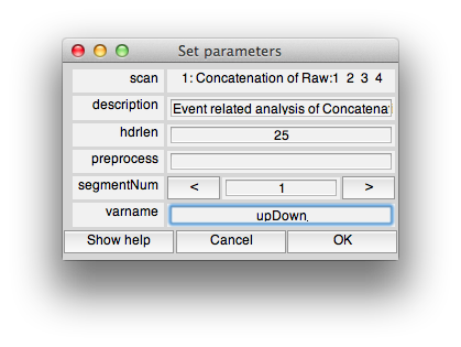
Now run an event-related analysis (Analysis/Event Related Analysis) and use all the default options until you get to the following dialog box in which you will set the varname to upDown (Note that it is really important to put the variable name “upDown” into the dialog box otherwise it won't know what variable to compute event-related analysis for):
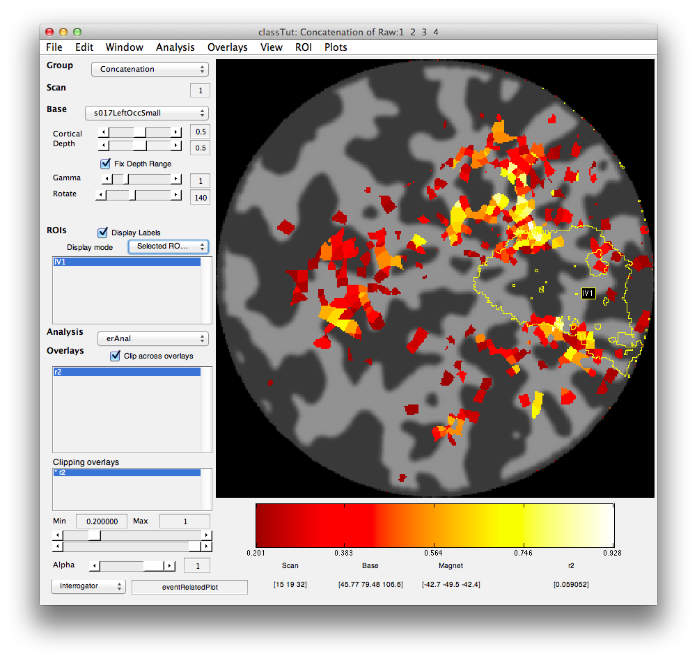
Set the Clipping overlay Min (slider or text box in bottom left) to 0.2) and then switch the Base (drop-down in top left) to display the left occipital cortex flat patch (s017LeftOccSmall). You should see a map of the r2 values that looks like the following.
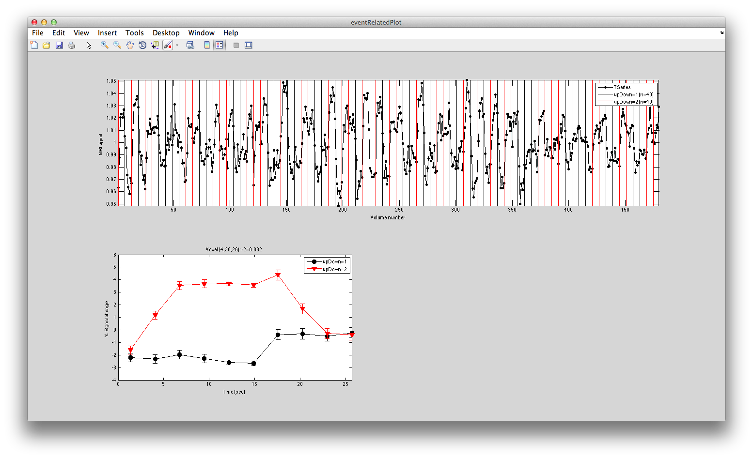
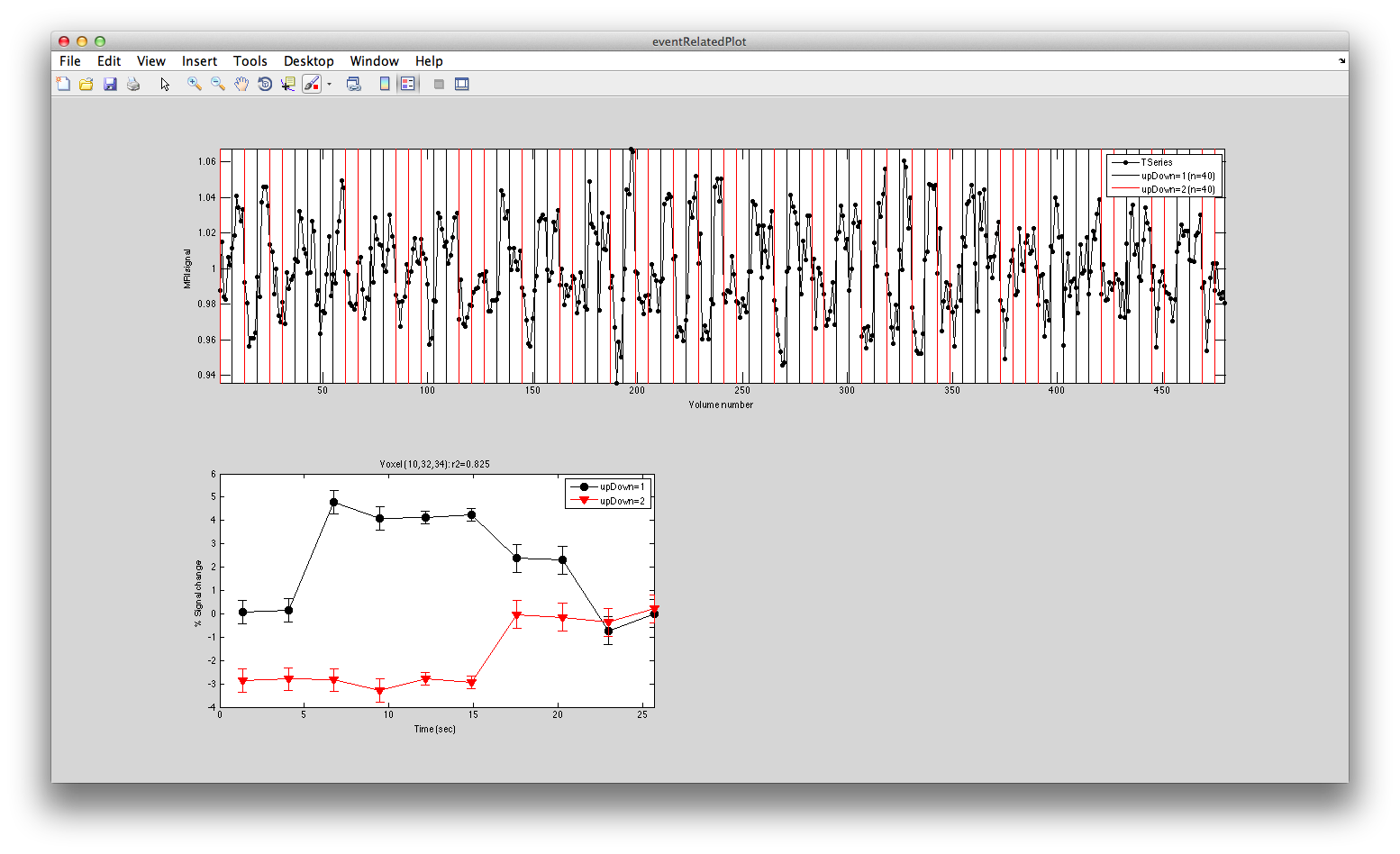
Turn on the interrgator (Plots/Interrogate Overlay) and click on a few points in the top using the eventRelatedPlot and you should see something like this:
Clearly larger responses for the trials when the stimulus was in the lower visual field, just as is expected for the topographic representation in early visual cortex. Clicking on voxels at the bottom, you should see this pattern reversed.
Classification analysis
Now, it should be quite easy to build a classifier, right? Just by seeing whether voxels that represent the upper visual field are responding or the ones that represent the lower visual field are responding we should be able to predict where the stimulus was. Let's train a classifier to do this.
We need to get the instances of responses for each stimulus type. That is, we want a number representing the response to each trial from each voxel in an ROI. Let's do this for the left V1. Load the lV1 ROI from File/ROI/Load
You should see the ROI like this (check that Selected ROIs (Perimeter) is selected in the Display Mode drop down in the middle left.
Note that the voxels with high r2 are right at the top and bottom of V1 just as expected (since that is where the lower and upper visual meridians are represented).
Now go to the Matlab command line and use getStimvol to get the stimvols for the upDown stimulus. That is, we want to know which volumes in the scan each stimulus began at. That is what is put into stimvol. Stimvol is a cell array with two elements. The first is all the stimvols for when the stimulus was in the upper visual field, and the second when the stimulus was in the lower visual field.
>> stimvol = getStimvol(getMLRView,'upDown')
(getStimvolFromVarname) taskNum=[1], phaseNum=[1], segmentNum=[1]
(getStimvolFromVarname) upDown=1: 10 trials
(getStimvolFromVarname) upDown=2: 10 trials
(getStimvolFromVarname) taskNum=[1], phaseNum=[1], segmentNum=[1]
(getStimvolFromVarname) upDown=1: 10 trials
(getStimvolFromVarname) upDown=2: 10 trials
(getStimvolFromVarname) taskNum=[1], phaseNum=[1], segmentNum=[1]
(getStimvolFromVarname) upDown=1: 10 trials
(getStimvolFromVarname) upDown=2: 10 trials
(getStimvolFromVarname) taskNum=[1], phaseNum=[1], segmentNum=[1]
(getStimvolFromVarname) upDown=1: 10 trials
(getStimvolFromVarname) upDown=2: 10 trials

stimvol =

    [1x40 double]    [1x40 double]
This shows you that there were 10 trials of each in each of the four component localizer scans for a total of 40 instances of each response type.
Now that we know the stimvols we need to get the responses to each stimulus presentation. We are going to do this by averaging the response in the time series for each of the voxels in left V1 across the time when the stimulus was presented (actually we time shift by a few seconds to account for the hemodynamic lag). First load the time series for lV1:
>> lV1 = loadROITSeries(getMLRView,'lV1')
(loadROITSeries) Loading tSeries for lV1 from Concatenation: 1 took 0 secs 766 msmin 00 sec)

lV1 =

         color: 'magenta'
        coords: [4x5397 double]
          date: '05-Jul-2013 12:57:25'
          name: 'lV1'
         notes: ''
     sformCode: 1
      viewType: 'Volume'
       vol2mag: [4x4 double]
       vol2tal: []
     voxelSize: [1 1 1]
         xform: [4x4 double]
       scanNum: 1
      groupNum: 2
    scanCoords: [3x200 double]
             n: 200
       tSeries: [200x480 double]
Now in the field tSeries you have the time series (480 volumes) for each of the 200 voxels that we have in left V1. We next set a sort order. This is used in times when you are only going to use a subset of your voxels in the classification (for example, you may want to use only a one hundred not the full two hundred to equalize ROI size across idfferent visual areas). But, which voxels to use. The sort index tells the programs what order to use. For right now, we don't care cause we are going to use all the voxels in the ROI, so let's just set this to the order the voxels happen to be in the ROI:
lV1 = getSortIndex(getMLRView,lV1);
We now need to snip this up into the pieces of response after each stimulus presentation and average for the duration of the stimulus. We use getInstances:
>> lV1 = getInstances(getMLRView,lV1,stimvol,'n=inf')
(getInstances) Creating 40.0 instances for lV1 with Inf voxels by taking mean from vol 1:6 (2.70s-16.20s) took 2 secs 174 msmin 00 sec)
took 2 secs 174 ms

lV1 =

    [1x1 struct]
Note that getInstances turned lV1 into a cell array (usually we run in on multiple ROIs, so let's just turn it back into a single ROI:
lV1 = lV1{1};
Now, we can grab the instances from the ROI which is stored under the classify field:
>> i = lV1.classify.instances

i =

    [40x200 double]    [40x200 double]
So there are 40 instances of response for each category (stimulus up or stimulus down) and each instance is a 200 dimensional vector (1 dimensional for each voxel - compare to above where we just had 2 dimensions).
Well, we can just run leaveOneOut on this and see how we do:
>> leaveOneOut(i)
(leaveOneOut) Class 1 has 40 instances with 200 dimensions
(leaveOneOut) Class 2 has 40 instances with 200 dimensions
(leaveOneOut) fisher classifier produced 91.25% correct and took 10 secs 449 ms

ans =

                type: 'fisher'
    classifierParams: [1x1 struct]
          whichClass: {1x2 cell}
       classifierOut: {[1x40 double]  [1x40 double]}
     confusionMatrix: [2x2 double]
             correct: 0.9125
          correctSTE: 0.0315918798902503
91% correct is not bad. Note that this is defaulting to using fisher linear discriminant.
So, great. We can classify the stimulus what does that mean? Well it means that there are responses that are specific to whether the stimulus was presented above or below just as expected.If there was nothing useful, this number would hover around 50% and you would know that there probably is nothing very interesting in your data with respect to the variables you are trying to classify.
Weight maps
It is a good idea for any classification you do, to check to see what the spatial arrangement of voxels is that allows the classifier to work. Let's look at this. First lets prepare the ROI by setting its sortIndex (more on this later - but, for now we just set dummy values)
>> weightMap = getClassifierWeightMap(getMLRView,lV1,stimvol);
(getInstances) Creating 40.0 instances for lV1 with Inf voxels by taking mean from vol 1:6 (2.70s-16.20s) took 2 secs 114 msmin 00 sec)
took 2 secs 114 ms
(buildClassifier) Building fisher classifier for ROI lV1 took 0 secs 105 msmin 00 sec)
What this did was build a classifier to classify the stimulus classes in stimvol using all the voxels in the ROI (no cross-validation) and it returns the weightMap.
Now weightMap contains the map of weights for each voxel in the ROI (actually it has the same dimensions as the scan 64x64x38 where values with a weight calculated are set to that weight and all other values contain NaN).
Now let's display it: First drop the erAnal analysis that you are currently viewing by doing View/Remove Analysis. Now from the command line do:
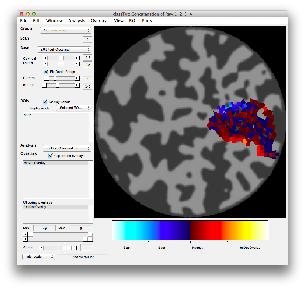
mrDispOverlay(weightMap,lV1.scanNum,lV1.groupNum,getMLRView,{'up vs down'},'colormapType','normal','cmap',splitcmap,'range=[-9 9]','clip=[-9 9]');
You should see the following:
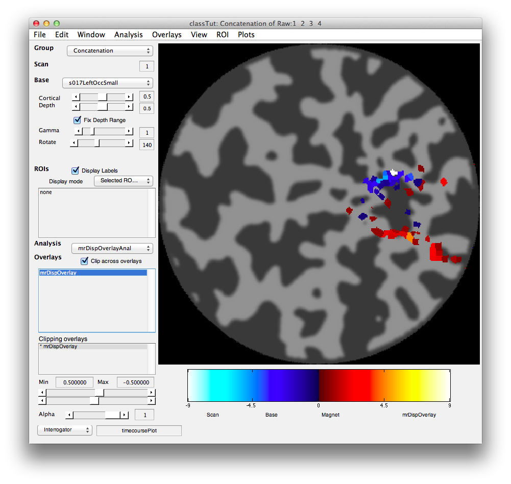
You should see that negative weights are near the top and positive weights near the bottom. This is exactly what we expect based on the topography. Voxels that have a larger response for the stimulus when presented at the bottom have negative weights and voxel with larger responses for when the stimulus was presented at the top have positive weights. You can see this more clearly, but clipping out all the weights that are in the middle ranges. This is done by crossing the min/max ranges of the Clipping Overlay (bottom left). That is, set the min to 0.5 and the max to -0.5 and you should see the following:
Clearly the voxels that have high weights (contribute information to the classifier) are all just where we expect them to be at the upper and lower parts of V1 that represent the vertical meridians where the stimuli were placed.
Number of voxels by accuracy plots
Sometimes it is interesting to know how much better performance of the classifier gets as a function of how many voxels enter the analysis. If only a few voxels are needed it suggests strong selectivity - if you need many it suggest weak selectivity in a large distributed pattern. If you add too many voxels you might just be adding noise and performance can decline. So, let's see what happens with this data set.
First we have to decide what order to include voxels in the analysis. This is a very important step. Typically what we do is use an independent localizer of some sort (perhaps retinotopy) to define which voxels we think will have a stimulus driven response. In this case, we are going to cheat a little and use the r2 from the event-related responses. This is cheating because it is a violation of cross-validation (choosing which voxels to use on data from the test set) - we should really choose voxel using data only from the training set or better yet a completely independent data set so that we don't break cross-validation.
But, with that in my mind, we need to get the r2 values from the event-related analysis. Going to the GUI and remove the mrDispOverlay analysis of the classifier weights (View/Remove Analysis). Now go load the erAnal analysis File/Analysis/Load load erAnal/erAnal.mat
Then from the command window get the r2 values of the overlay:
r2 = viewGet(getMLRView,'overlayData',1);
Now we are going to set the sort order according to this r2 map (remember before we just set the sort order to the random order that the voxels happen to be in the ROI):
lV1 = getSortIndex(getMLRView,lV1,r2);
Now, let's compute leaveOneOut classification performance as a function of how many voxels we use. This may take a few minutes to compute:
voxNums = [1:20:lV1{1}.n];
correct = [];
for nVox = voxNums
  lV1 = getInstances(getMLRView,lV1,stimvol,'n',nVox);
  instances = lV1{1}.classify.instances;
  l = leaveOneOut(instances);
  correct(end+1) = l.correct;
  disp(sprintf('%0.2f%% correct with %i voxels',100*correct(end),nVox));
end
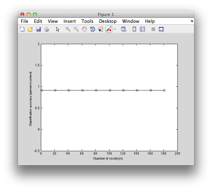
Now if we plot it, we can see that basically we always get the best performance even if we use 1 voxel!
plot(voxNums,correct,'ko-');
xlabel('Number of voxels (n)');
ylabel('Classification accuracy (percent correct)');
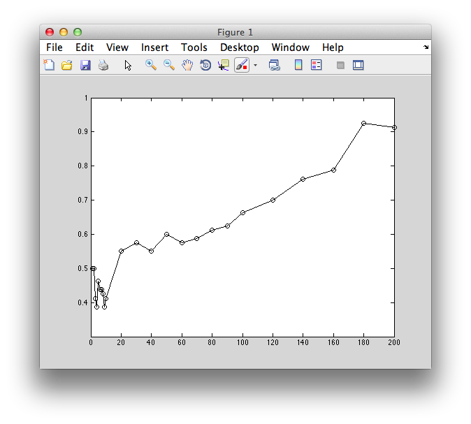
Just to prove that the order matters, let's reverse the sortindex so that now the worst voxels (in terms of how much they respond to the stimulus - not necessarily how well they differentiate between stimuli) are first.
lV1{1}.sortindex = fliplr(lV1{1}.sortindex);
Now do the classification again:
 voxNums = [1:2:10 20:10:100 120:20:lV1{1}.n];
correct = [];correctSTE = [];
for nVox = voxNums
  lV1 = getInstances(getMLRView,lV1,stimvol,'n',nVox);
  instances = lV1{1}.classify.instances;
  l = leaveOneOut(instances);
  correct(end+1) = l.correct;
  correctSTE(end+1)
end
Now you only get good performance when you add the best voxels back.
plot(voxNums,correct,'ko-');
xlabel('Number of voxels (n)');
ylabel('Classification accuracy (percent correct)');
Classify by hand
Just for fun, let's see if we can classify the data by hand. Let's get the instances again for two voxels:
lV1 = getSortIndex(getMLRView,lV1,r2);
lV1 = getInstances(getMLRView,lV1,stimvol,'n=2');
instances = lV1{1}.classify.instances;
Now we can plot the points:
classifyTest(instances{1},instances{2},'tightAxis=1','type=none')
And we can try the mean classifier:
m1 = mean(instances{1});
m2 = mean(instances{2});
w = m2-m1;
classifyTest(instances{1},instances{2},'tightAxis=1','w',w);
Already that does well. As an exercise try it with naive-bayes or fisher or svm and see what you get.
Dimension reduction with PCA then classification
We can also try to build with all 200 voxels:
lV1 = getInstances(getMLRView,lV1,stimvol,'n=inf');
instances = lV1{1}.classify.instances;
But then it is hard to visualize all 200 dimensions so we need to project into a smaller space. We could do this in many ways. Some people do this as a first step to classification to get rid of noise, but its risky. Which dimension is the best dimension for classification? It could be dimensions that have the most variance in them - but that variance may not be associated with responses that are different for different categories. Nonetheless, we project onto these dimensions - the ones that account for the most variance in the data. We can do this by using PCA:
pcaBasis = pca([instances{1};instances{2}]);
This is essentially a rotation of the data space so the orthogonal axis point in directions of most variance within the data. We take the top two dimensions and project our data down on to those dimensions:
for iNum = 1:40
  x1(iNum,1) = dot(instances{1}(iNum,:),pcaBasis(:,1)');
  x2(iNum,1) = dot(instances{2}(iNum,:),pcaBasis(:,1)');
  x1(iNum,2) = dot(instances{1}(iNum,:),pcaBasis(:,2)');
  x2(iNum,2) = dot(instances{2}(iNum,:),pcaBasis(:,2)');
end
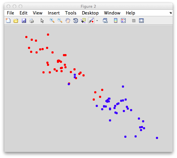
Then the data in these two dimensions look like this:
classifyTest(x1,x2,'tightAxis=1','type=none')
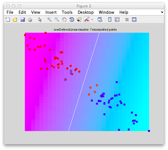
And classifying using Fisher like this:
classifyTest(x1,x2,'tightAxis=1','type=fisher')
We get:
Classification tools
-jg.
