Table of Contents
Preprocessing analyses
Preprocessing analyses are ones that create new time series. They are usually run before you run other analyses steps like correlation analysis and event-related processing.
Motion Compensation
Motion compensation in mrLoadRet-4.5 uses the same computational engine of mrAlign. To access the motion compensation window go to the menu:
The window will let you:
- Choose the Group to which motion compensation should be applied.
- Choose the type of interpolation (how pixels on two images will be will be chosen for alignment).
- Crop the image (clicking the crop button will bring up a new window on which to choose the first and last slice utilized for cropping and will let you crop the image). Note that the images ARE actually cropped when computing the alignment and that the same crop region is used for contrast correction also.
- Correct the image for contrast/intensity (see below).
- Do time slice correction. If you choose to do slice time correction, then mrLoadRet will resample the data in time to correct for the fact that the different slices were acquired at different times during each TR. This can make a noticeable difference when precise timing is desired.
This option is reccommended for 2D acquisitions only (not if you are using the spiffy 3D EPI pulse sequence). Furthermore, It is important to have some junk frames at the beginning and at the end of your protocol (at least 3)
- Choose the scan to motion correct. Standard parameters for 3X3X3 cbi epi scans motion compensation are:
- Interpolation method: cubic
- Number of iterations: 3
- Robust: NO (Unclicked, unless your scan session has both online and raw files; see below)
- Crop: just remove a little bit of background around the images (it runs faster) N.B. The overall motion compensation process is long (nearly 1hr per scan on a MacPro 2 X 2.66 GHz Dual-Core Intel Xeon with 3GB of RAM) it is convenient to invoke files from your local drive (i.e., copy data files and mrTools-4.5 files to local directory before invoking dofmrinyu, otherwise any network error could stop the procedure)
Notes on intensity correction and robust estimation
Some more facts about these two options to help you decide when to use them:
Intensity Correction
Pros: corrects for intensity differences due, e.g., to coil placement, saturation bands, etc. Cons: blurs the data to do the calculation. Reasons to use it: If the scans you are correcting come from different scanning days, or were taken with different acquisition parameters (e.g. raw and online), or have different voxel sizes, etc. Or if you're measuring hi-resolution data (because the saturation bands cause the signal to go to zero, and that big signal change will swamp out any smaller signal changes due to motion, making it impossible to measure or correct the motion-induced signals; the same goes for using 3D EPI sequences, because the signal in the first and last slices will go to zero). Important Note: If you use the intensity correction, you want to choose a crop region that is largely inside the brain so that it is the signal from within the brain that is used to calculate the correction.
Robust Estimator
Pros: Less sensitive to outliers. Cons: prone to local minima and other problems of non-linear estimation, as compared with least-squares. Reasons to use it: If you have reason to believe your data suffers from outliers. In general, for all the problems listed above, you will use the intensity correction, but that correction does not work perfectly, and you may still be left with noisy outliers that you need to ignore in order for the motion compensation to succeed.
Average Time Series
This step allows you to average the time series for two or more scans. For example, if you are analyzing retinotopy data, you will want to average the expanding and contracting rings (with one reversed), and to average the rotating wedges (eg CW and reversed CCW). Or, for any other experimental design in which you had repeated scans (eg so as to reduce noise). Also, for averaging across subjects, or across days within the same subject.
Computes average of the time series. Time reverses and shifts as specified. Output is a new tSeries file added to the specified group, and that is in the coordinate frame of the base scan.
Order of operations is:
1) dump junk frames,
2) time shift,
3) time reverse,
4) average (transforming to coordinate frame of the base scan).
Using the function with the GUI
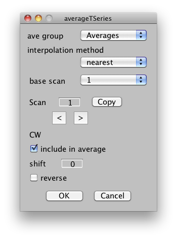
When you choose averageTseries from the Analysis menu, you will see a box like this:
The choices you have when using the GUI correspond to the choices you have for the parameters listed below, so they are not repeated here.
Once you hit 'ok', the average will be computed and will be added as a new scan to the indicated group.
Using the function in scripts
When scripting, it can be called as follows: [view params] = averageTSeries(view,params,varargin)
The input 'params' is optional (default: user is prompted via averageTSeriesGUI). If it is provided, it must be a structure with all of the following fields:
| fields | notes |
|---|---|
| scanList | Vector of scan numbers to include in the average. Default: all of the scans. |
| tseriesfiles | Cell array of strings the same length as scanList, specifying the tseries filenames. Or 'any' to allow any match with the tseries files. |
| shiftList | Vector of integers the same length as scanList, each entry of which specifies the time shift (in frames, i.e., 1 means a shift of 1TR) for each scan. Default: all zero (no shift). |
| reverseList | Vector of the same length as scanList with non-zero entries indicating which scans to time reverse. Default: all zero (no time reversal). |
| baseScan | Number specifying scan which is used to specify the coordinateframe for the result. Default: first scan. |
| interpMethod | 'nearest', 'linear', 'cubic', or 'spline' as in interp3. |
| groupName | Group of scans that will be averaged. Default: current group of view. |
| aveGroupName | The new average scan is added to the specified group. If the group specified by aveGroupName does not exist, then a new group is created with this name. Default: 'Averages'. |
| description | Description string for the new average scan Default: 'Average from <groupName>' of scans: <scanList>'. |
| fileName | The new tseries is saved in the specified filename. Default: 'tseries-mmddyy-hhmmss.img' or 'tseries-mmddyy-hhmmss.nii' where mmddyy = date and hhmmss = time. Chooses between .img and .nii, based on 'niftiFileExtension' preference. |
This function also saves an auxillary file (tseriesfileName.mat) that can be used to % recompute as follows:
load FileName.mat
eval(evalstr)
Examples:
params = averageTSeriesGUI('groupName','Raw');
view = newView;
view = averageTSeries(view,params);

view = averageTSeries(view);
Concatenate Time Series
This step will take the scans you select, get rid of any junk frames, do a de-trending step using a hi-pass filter if you specify that, and then concatenate the resulting time series into a single time series that will be saved into a new group called Concatenation. This is an essential step if you plan to analyze data that was run over many consecutive scans.
Note that the concatenation code will keep track of many things for you: It will throw out the junk frames, but keep track of how many frames have been thrown out. It will internally make the timing consistent, so your stimulus timing files should be with reference to the original raw timing. For example, if you have a TR of 2 seconds, and have 5 junk frames at the start of each scan, and only begin your experimental protocol on the 6th time frame, your stimulus timing should reflect that the first stimulus is shown at 11 seconds, not 1 second.
Also note that the hi-pass filtering that is done here is a different function call from the filtering done in other parts of the code, such as percentTSeries.m, and the filter cutoff is referenced differently. For the concatenation code, the hi-pass filter cutoff is set in Hz (default 0.01 Hz) and in percentTSeries it's set in cycles/scan. It will also make the mean of your time series 1, that way if you try to divide by the mean again, it won't cause an error.
After concatenation, concatTSeries saves a structure that gives you information about the concatenation. You can access that with a viewGet:
v = newView;
concatInfo = viewGet(v,'concatInfo',1,'Concatenation');
It has the following fields:
>> concatInfo
concatInfo =
                n: 8
        whichScan: [1x1536 double]
      whichVolume: [1x1536 double]
            nifti: [1x8 struct]
         filename: {1x8 cell}
             path: {1x8 cell}
       junkFrames: [0 0 0 0 0 0 0 0]
     hipassfilter: {1x8 cell}
    runTransition: [8x2 double]
concatInfo.whichScan tells you the number of the scan each volume came from. It has length the number of volumes in the concatenation (1536 for this case). whichVolume tells which volume of the original scan the volume came from. nifti, filename and path tell you the nifti header, filename and path of each original scan. junkFrames keeps the junkFrames of each original scan. hipassfilter is a cell array of filters that were used (it stores the fourier coefficients of the filter used). runTransition is an array which tells you where the run transitions happen, i.e. for each scan, the first column gives you which volume that scan starts at and the second column gives you which volume that scan ends at.
Postprocessing analyses
Correlation Analysis
Using the GUI
This allows you to calculate how well each voxel's timecourse correlates with a given modulation. This is useful for analyzing localizers, block-design experiments, and retinotopy experiments.
Take retinotopy, for example. After averaging the appropriate scans, you have a group ('Averages') with two scans, one with the timecourses related to the rotating wedges and the other with the timecourses related to the expanding rings.
Next, you compute a correlation analysis, so that you can visualize the cortical responses to the stimuli.
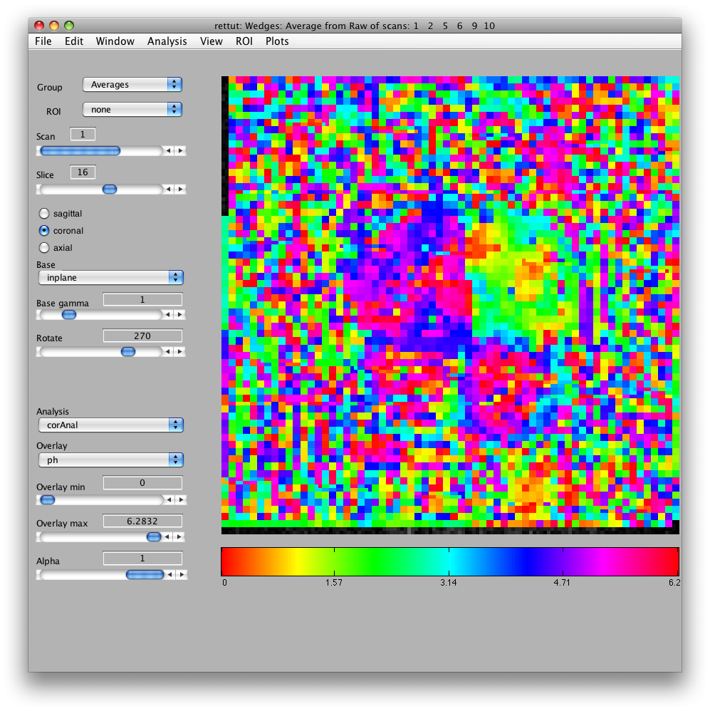
To run the correlation analysis from the GUI, choose the menu item Analysis/Correlation Analysis. For both scans, you will select (re)compute and set the number of cycles to 10. It should look like the following:
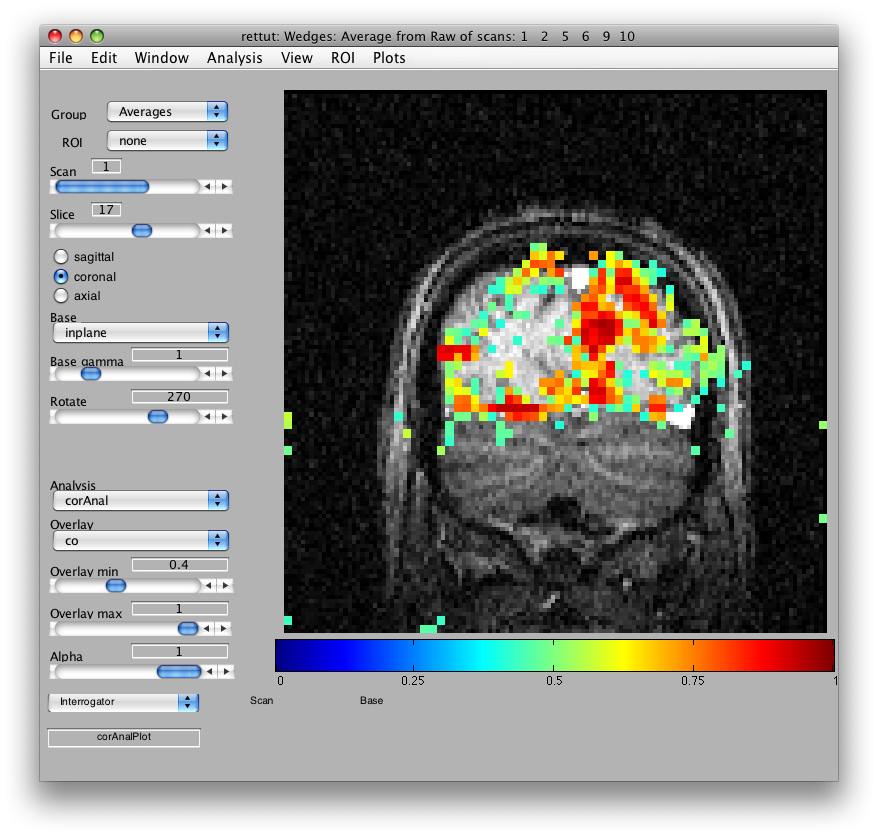
When it has finished running, you should see something like this:
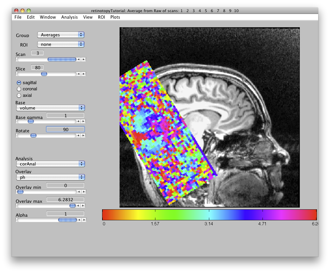
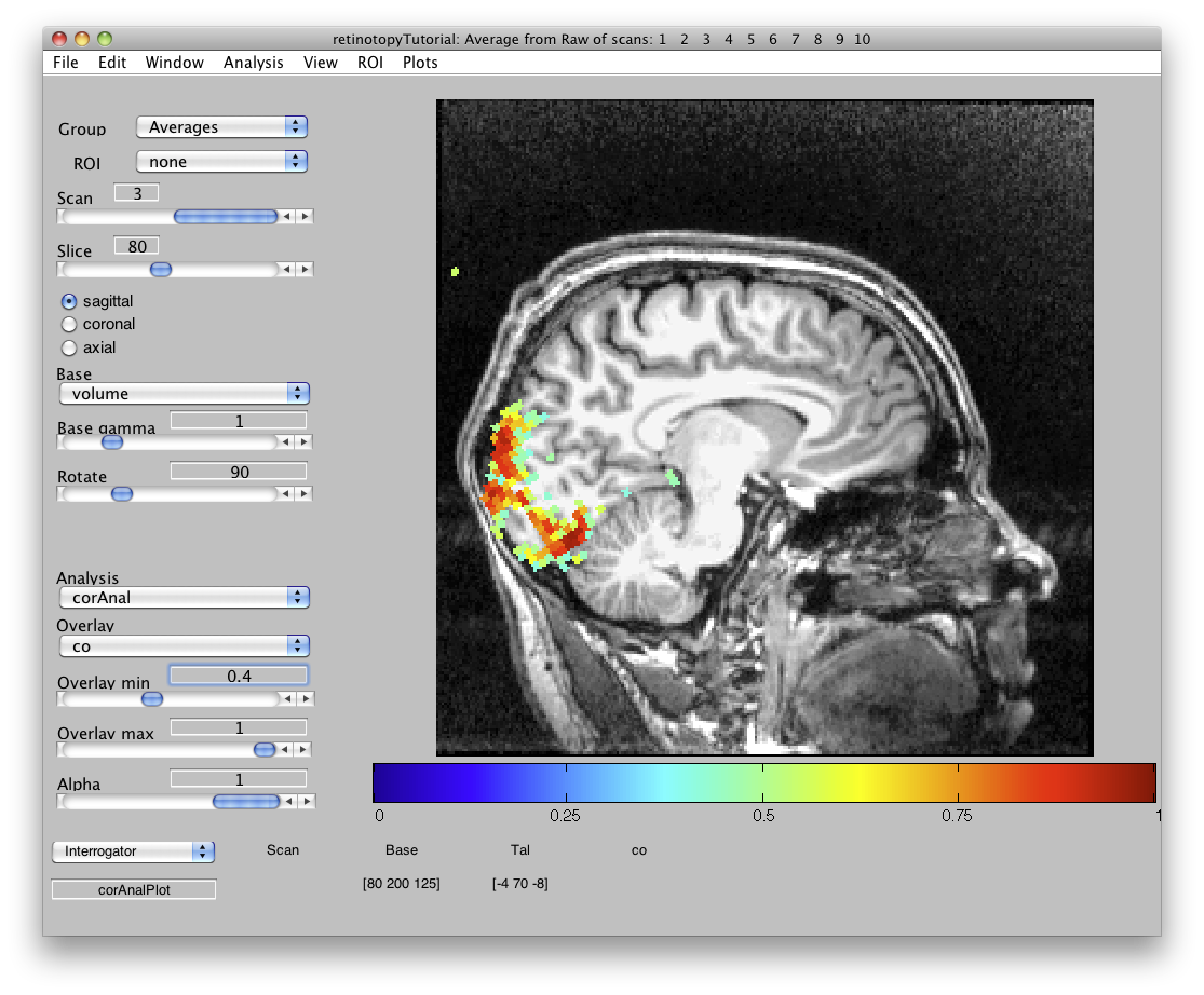
or this (viewed on the volume rather than on the EPIs):
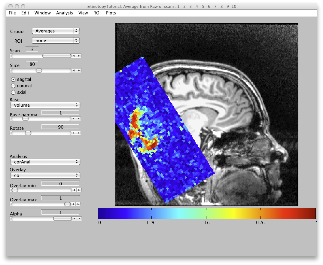
Notice that under the 'Analysis' tab on the bottom left hand corner of the mrLR screen, 'corAnal' is showing. Underneath the name of the analysis, is the name of the overlay currently showing. The correlation analysis creates three overlays:
ph: phase co: coherence amp: amplitude
The co map gives a sense of which voxels were responding to the visual stimulus:
Now, let's try to examine single voxel responses on the map.
You can set the Overlay min to 0.4 so that you are only looking at voxels with a high correlation value.
Then turn on the voxel interrogator, by going to Plots/Interrogate Overlay. You should see something like this:
(Or like this, viewed on the EPIs:)
Note that now, an Interrogator drop down has appeared in the lower left of the viewer and that it is pre-set to corAnalPlot.
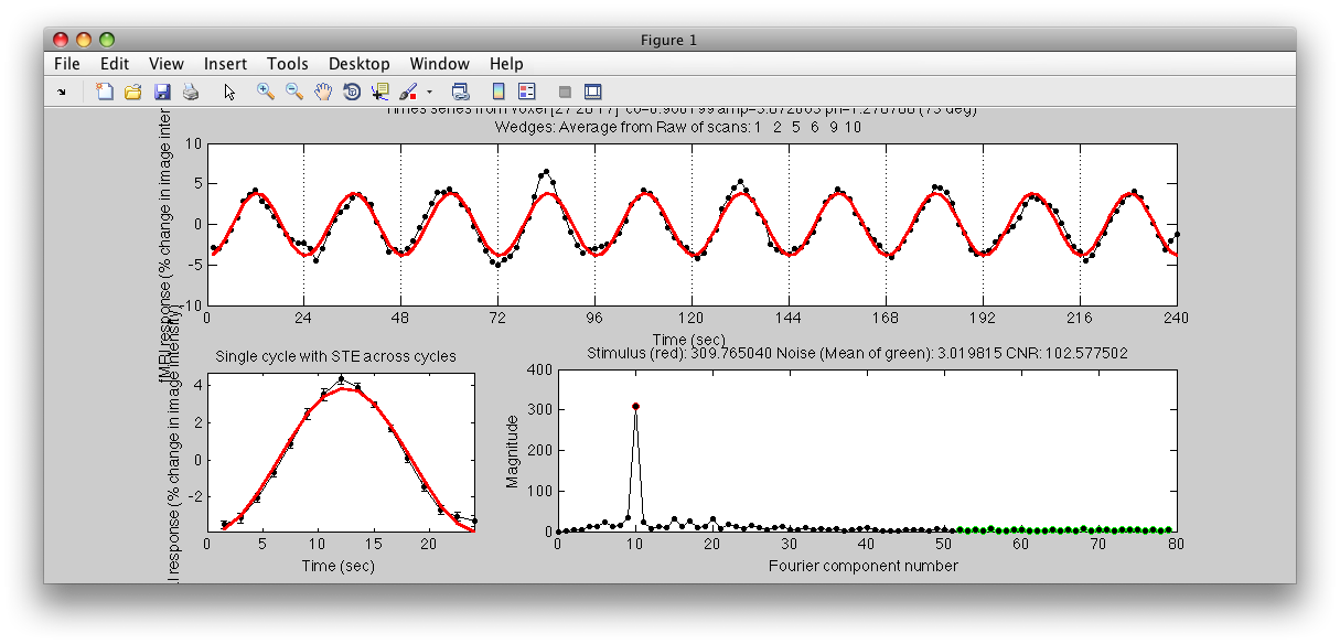
When you move your mouse over the image it should now turn into a giant cross-hairs. Choose one of the voxels (the example below is voxel [27 28 17]) with the darkest red color and click. After a moment, you should see a figure like this:
Looks very well modulated at the stimulus frequency! Contrast-to-noise ratio (i.e. the magnitude of the response at the task frequency (marked in red in the lower right graph, divided by the mean of the points marked in green) is over a 100-to-1.
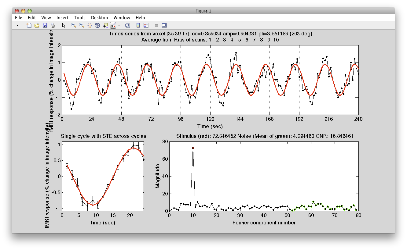
Another voxel's data may look like this: (for voxel [35 39 17])
Accessing the output
You can access the analysis using viewGet:
v = newView;
corAnalysis = viewGet(v,'analysis')
The analysis structure has the following fields:
             curOverlay: 1
                      d: {[]  []  []}
                   date: '23-Nov-2010 15:24:33'
               function: 'corAnal'
              groupName: 'Averages'
            guiFunction: 'corAnalGUI'
          mergeFunction: 'corAnalMergeParams'
                   name: 'corAnal'
  overlayInterpFunction: 'corAnalInterp'
               overlays: [1x3 struct]
                 params: [1x1 struct]
      reconcileFunction: 'corAnalReconcileParams'
                   type: 'corAnal'
You can access each overlay (co, ph, and amp) using viewGet as well:
v = newView;
ov = viewGet(v,'overlay',[overlayNum],[analysisNum])
You can see which overlays are provided by the analysis as output:
>> viewGet(v,'overlayNames')
ans =
  'co'    'amp'    'ph'
You can also access each overlay by name:
amp = viewGet(v,'overlay','amp')
The overlay has these fields:
amp =
                 alpha: 1
          alphaOverlay: []
  alphaOverlayExponent: 1
                  clip: [8.9680e-04 219.4702]
              colormap: [256x3 double]
          colormapType: 'normal'
                  data: {1x3 cell}
                  date: '23-Nov-2010 15:24:33'
              function: 'corAnal'
             groupName: 'Averages'
          interrogator: 'corAnalPlot'
         mergeFunction: 'corAnalMergeParams'
                  name: 'amp'
                params: [1x1 struct]
                 range: [8.9680e-04 219.4702]
     reconcileFunction: 'corAnalReconcileParams'
                  type: 'amp'
Event Related Analysis
The event-related analysis done in MLR uses deconvolution to compute the estimated response to each stimulus type. There is a tutorial that will help familiarize you with how it works.
Any event-related analysis starts with the timing of the events. There are a few different ways to get the information about timing events for your scan:
- MGL stimfiles If you are using the mgl task code then you will get “stim” files that are associated with each run. These contain all the information about the experiment that you ran and can be used directly by MLR to calculate stimulus times in a variety of different ways.
- stimvols This is perhaps the simplest way to save your stimulus times. You make a matlab cell array called stimvol and each element in the cell array is an array which contains the volume numbers when each event occurred. For example, if you had an experiment in which you had two trial types, A and B, and they occurred on stimulus volumes 1, 10, 40 and 25, 55, 75 respectively, then you would have:
stimvol = {[1 10 40],[25 55 75]};and you would save the file as:
save stimFilename stimvol
- Time log These files contain a variable mylog which should have the field mylog.stimtimes_s and optionally the field mylog.stimdurations_s. The field mylog.stimtimes_s should be a cell array, with length = number of conditions. Each cell should be a vector of times, in seconds, indicating the time of the stimulus onset for that condition. The vectors do not need to be the same length (e.g. if you have different number of trials for the different conditions). Optionally, you can also specify mylog.stimdurations_s, with a duration value to correspond to each onset time for each stimulus in each condition. A sample, with two conditions, one occurring at 0, 15.3 and 32 seconds and the other at 11 and 24 seconds, would look like the following:
  mylog.stimtimes_s = {[0 15.3 32],[11 24]};
  save stimFilename mylog
For both stimvols and Time log you can add a variable named stimNames to the .mat files. If stimNames exists, then it will be used by eventRelatedPlot to label of different conditions. For example, if you had three different conditions named “Type 1”, “Type 2” and “Type 3”:
stimNames = {'Type 1' 'Type 2' 'Type 3'};
And you would save it (if it were stimvols) like:
save stimFilename stimvol stimNames
Whatever format you use for your files in you should save them in a folder named Etc in your session directory. You can then link them to each scan, using the GUI item Edit/Scan/Link Stimfile. Note that you should always link the stim files to the raw time series. You do not have to link them before you concatenate the time series. MLR keeps track of where each scan originally came from and works backwards to find out what the stim files are. So if you change the stimfile linkage at some later time, you do not need to relink the stim files.
Once you have the stimfile linked properly, you can run the event-related analysis. Typically, one does an event-related analysis on a concatenated time series. This is true even if you only have one scan, since the concatenate time series takes care of the high-pass filtering of your data. The event-related analysis is done by making a stimulus convolution matrix from your stimvols. You need to choose how many volumes that you want to compute out the response for (hdrlen). Then the code will create a “Toeplitz” matrix (a matrix in which the all diagonals contain the same number) where all the stimulus volumes in the first column are set to 1. This is also known as a stimulus convolution matrix. For example, if you had a scan with 10 volumes and your events happened on the 1st and 7th volume and you were computing a hemodynamic response length of 5 volumes, the matrix created would look like the following:
In general linear model language this is the “design matrix”, and the solution is taken using the pseudo-inverse. The assumption that is made in this analysis is that if there is response overlay those response sum linearly; that is it is based on the assumption of temporal linearity. Evidence for temporal linear summation of BOLD responses has been reported in Boynton, Engel, Glover and Heeger (1996) J Neurosci 16: 4207-4221.
The code will also compute an r2 map which reports the amount of variance in the original time series that is accounted for by the event-related responses (see Gardner, Sun, Waggoner, Ueno, Tanaka and Cheng (2005) Neuron 47:607-620).
The standard error bars for the hemodynamic responses are computed by first getting the sum of sum of squares of the residual time course and dividing that by the number of volumes minus the number of responses x the hdrlen. This residual is then distributed to each time point in the estimated response according to the inverse of the covariance of the design matrix. These errors assume that the noise is white and gaussian. After high-pass filtering to remove low frequency signal changes and drift, this assumption is not completely unreasonable (look at the frequency spectrum of the residuals, it should be flat).
preprocess
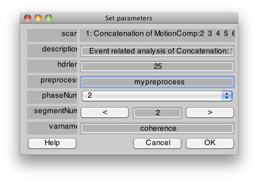
There are times when you may need to create stimvols in ways that are more complicated then a normal experiment. For example, you may want to sort your trials by subject's responses. In these cases, you can either create your own stimvol array explicitly and save that as a file that you link the scan to (see above). You can also specify a preprocess function in the eventRelated gui:
The function you specify here can adjust the stimvols in any way that you want. It should be a function that takes a “d” parameter and returns a “d” parameter. Here is a very simple example which takes stimvols that specify a set of different stimuli (i.e. is a cell array of k different arrays specifying stimvols for each stimulus condition) and collapses that into a single type (i.e. creates stimvols that will calculate the response across all different stimulus types):
function d = mypreprocess(d)

d.stimvol = cellArray(cell2mat(d.stimvol));
In principle, you can do whatever processing is necessary to create a stimvol field that you need. The d structure that is passed in contains information about your scan. It looks like:
d =

              ver: 4.5
          scanNum: 1
         groupNum: 3
      description: 'Concatenation of MotionComp:2  3  4  5  6'
               tr: 1.2
        voxelSize: [3 3 3.00000047683716]
            xform: [4x4 double]
          nFrames: 1875
              dim: [64 64 22 1875]
         filename: 'tseries-080222-192610.img'
         filepath: [1x88 char]
          expname: 'jg060918_mr4'
         fullpath: '/Volumes/eigenraid/data/nyu'
             data: [4-D double]
       junkFrames: [0 0 0 0 0]
            dicom: {[1x1 struct]  [1x1 struct]  [1x1 struct]  [1x1 struct]  [1x1 struct]}
         stimfile: {[1x1 struct]  [1x1 struct]  [1x1 struct]  [1x1 struct]  [1x1 struct]}
       concatInfo: [1x1 struct]
          varname: [1x1 struct]
        stimNames: {'1'  '2'  '3'}
          stimvol: {[1x88 double]  [1x88 double]  [1x88 double]}
    supersampling: 1
GLM Analysis
At this point, you should be using GLM_single from Kendrick Kay's group. This isn't build into MRtools, so you should run your own script. You can find an example here: https://github.com/joshmw/interp/blob/main/run_glmDenoiseInterp.m
Create stimFiles
To run the GLM analysis, you need to create stimulus files that have the timing information for your experiment.
You should have a separate stimFile for each scan. See above under Event Related Analysis for a description of possible formats.
Just like for the Event Related Analysis, you then need to let mrSession know that these stimFiles have been defined. This can be done through the GUI menu (Edit/Scan/Link Stimfile). You can manually link each scan to a matlab .mat file (make sure to save mrSession afterwards). Alternatively, this can be scripted using a code along the lines of:
mrGlobals, view = newView;
groupNum = viewGet(view,'groupNum','MotionComp'); % or whichever group you're concatenating
numScans = viewGet(view,'nScans',groupNum);
for iScan = 1:numScans
  stimFilename = ['stimFiles/stimFile_' num2str(iScan) '.mat'];
  view = viewSet(view,'stimFilename',stimFilename,iScan,groupNum);
end
saveSession;
(Note that if the 1st stimFile goes with the 2nd EPI file, you need to adjust the indexing appropriately.)
Concatenate your data
You can either do this through the GUI or in a script. See details above for more info about concatenating.
In the GUI: choose Analysis → Concatenate Time Series
To script: You have to set the parameters and then call the code. For example:
mrGlobals, view = newView;
params.groupName = 'MotionComp';                 % sets which group to take the scans from
params.newGroupName = 'Concatenation';           % sets the name of the group that results from the concatenation
params.description = 'Concatenation of [x...x]';
params.filterType = 1;
params.filterCutoff = 0.0100;
params.percentSignal = 1;
params.projectOutMeanVector = 0;                 % explicitly specify that you do/do not want to do this
params.warp = 0;                                 % should set warp to 1 if combining across days
params.warpInterpMethod = [];                    % choose (e.g., 'linear') if combining across days
params.scanList = [1:viewGet(view,'numscans',viewGet(view,'groupNum',params.groupName))];
view = concatTSeries(view,params);                          %actually do the concatenation
Run the glm analysis
You can either do this through the GUI or in a script.
If you want to adjust the analysis code to the needs of your particular situation, you need to do it in a script, not the GUI, but you can use the code that the GUI uses as a guide.
The outcome of this step will be an overlay (or multiple overlays, if you want) that can be viewerd in the GUI.
Time Series Statistics
This computes several maps/overlays: mean over time, median over time, std dev over time, max frame-to-frame difference, max difference between each frame and the median, and the mean divided by the stdev.
The structure can be accessed using viewGet, and has the following fields:
» viewGet(v,'analysis')
ans =
         curOverlay: 4
                  d: []
               date: '16-Nov-2010 12:48:37'
           function: 'timeSeriesStats'
          groupName: 'Raw'
        guiFunction: 'timeSeriesStatsGUI'
      mergeFunction: 'defaultMergeParams'
               name: 'timeSeriesStats'
           overlays: [1x6 struct]
             params: [1x1 struct]
  reconcileFunction: 'defaultReconcileParams'
               type: 'timeSeriesStats'
Individual overlays can be accessed by name, using viewGet:
>> viewGet(v,'overlay','mean')
ans =
                 alpha: 1
          alphaOverlay: []
  alphaOverlayExponent: 1
                  clip: [0 3.1737e+04]
              colormap: [256x3 double]
          colormapType: 'normal'
                  data: {1x10 cell}
                  date: '16-Nov-2010 12:48:37'
              function: 'timeSeriesStats'
             groupName: 'Raw'
          interrogator: 'timeSeriesStatsPlot'
         mergeFunction: 'defaultMergeParams'
                  name: 'mean'
                params: [1x1 struct]
                 range: [0 3.1737e+04]
     reconcileFunction: 'defaultReconcileParams'
                  type: 'mean'
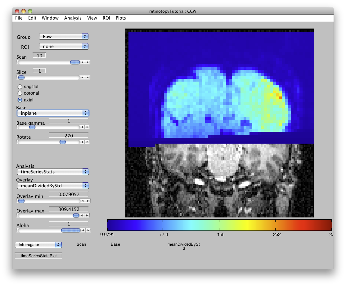
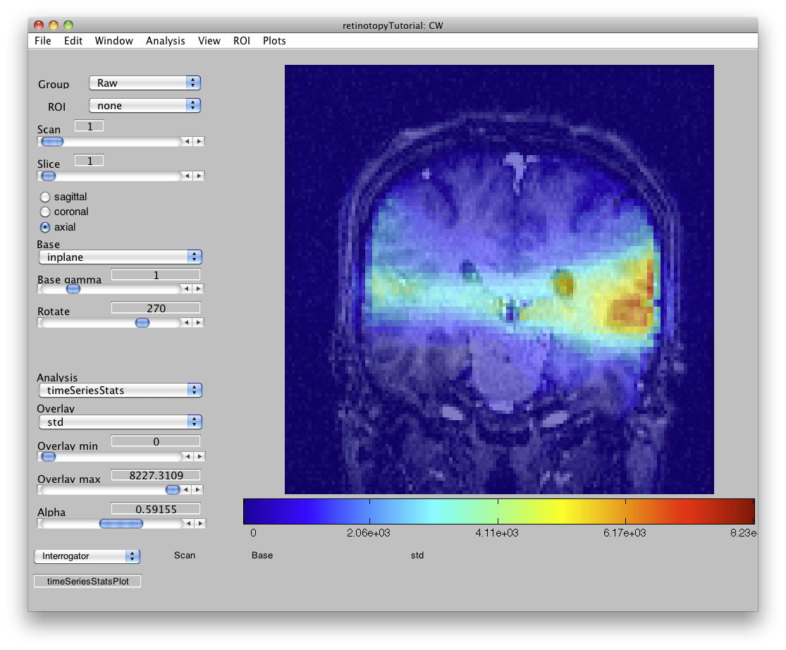
When the timeSeriesStats is loaded, you should see something like this:
- The mean map (and the mean/std map) of a successfully motion compensated group should line up well with the inplanes.
It is possible to check this by moving through successive scans (with the scan slider). They all should line up with one another.
- The median map should look similar to the mean map.
- The std map is a cheap way to find active brain regions without any knowledge of the experimental protocol.
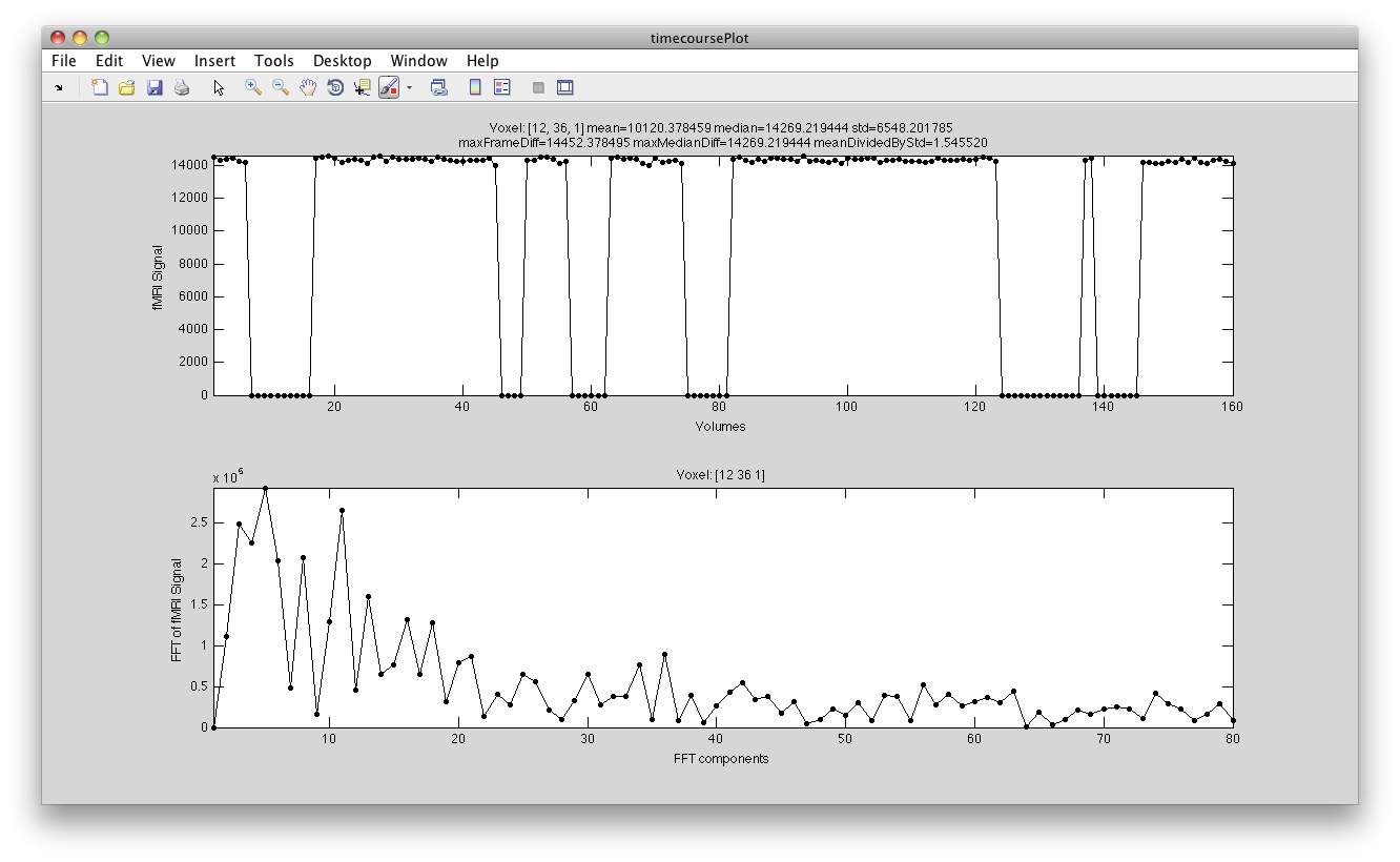
- If you go to Plots/Interrogate Overlay, the interrogator in the lower left hand corner will come up with a default plotter. When you select a voxel using the cross-hairs, you should see something like this:
- The max-frame-diff and max-median-diff maps are also useful for checking the motion compensation. Before motion compensation, these maps should show large values near the gray/white and gray/CSF boundaries because there are large intensity fluctuations over time due to motion. After motion compensation this “edge effects” should be largely eliminated.
