Table of Contents
Data processing, analysis and visualization with mrTools
This tutorial will guide you through data processing, analysis and visualization of your MRI data using mrTools.
Learning goals
After completing the tutorial you should be able to use mrTools to…
…examine raw data (epi and T1 weighted anatomies)
…determine whether motion-compensation worked
…examine the alignment between different data sets
…examine gray-matter / white-matter segmentations made by FreeSurfer and view surfaces
…find the calcarine sulcus and make flat patches of visual cortex
…average data and run pRF analyses
…determine the location of V1
…concatenate data and run an event-related analysis
Computer setup
In 2026, we're going to give you this already set up. At some point in the future, you might need these setup instructions. But for 2026 cog core, you can skip this section and proceed to the part about the raw data.
As of 2025, we've attempted to streamline this. You should have come to class with matlab 2019B installed, with the statistics and machine learning, financial, and image processing toolboxes downloaded.
You've been given two files - a data folder, named something like “s0xxx” (where xxx is your subject ID), and a software file, called “tools”. You should put both of these on your desktop. We've coded up mrTools to look for files there, so it should work if everything is in the right place.
Launch matlab. Then, in the command window, type:
>> cd ~/Desktop/tools
>> addpath(genpath(pwd))
This will add the software you need to your matlab path, so it can be executed. Then, you can:
>> cd ..
>> cd s0xxx
>> cd s0xxx20250410
again, where xxx is your subject ID.
Examine raw data
No matter what kind of experiment you do - you always want to look at the data you collect in as raw a format as you can. With neuroimaging this is even more important, because often data are processed with complex multi-step analyses and you can lose track of what features of your data give a result and get into real trouble. Lukily with imaging data, you can just look at your data, cause, well, it's a bunch of images. So let's do that first!
First, run program mrLoadRet in your data directory (you should have just moved into here in the step above). It will bring up a viewer. First thing to note is the “Group” drop-down at the top-left. We store data in different “groups” (folders on the harddrive) depending on what stage of analysis the data is in. We want to look at the “Raw” group - so:
Step 1: Select the “Raw” group
In MRI measurements there are different images made with different contrasts (for example, T1 or T2 or T2*-weighted images). For this purpose, just know that a typical anatomical image that you might see is “T1-weighted” where gray matter is gray, white matter is white and cerebral spinal fluid is black. You can take a look at that image by loading it as a “Base Anatomy”. A note here is that we can display summary statistics and data on many different kinds of base anatomies (we will see surfaces and flat-maps in a second). When we do so, we are just doing this for visualization - we transform the statistics on the fly to display on these base anatomies - we always keep the raw data in its original format (thereby avoiding messing with the original data too much by resampling and interpolation only when it is necessary to visualize). We always collect a T1 weighted anatomical image every session - this is used for visualization and for alignment with a canonical anatomy and surfaces (as we will see below).
Step 2: Load the T1 anatomy The anatomy should already be loaded into your session. In fact, if Josh set this up right (don't bet money on this [don't worry, Josh is writing this bit]), you should already be looking at it. If you aren't, go to the options on the left, and under “Base”, click the “anat01_T1w…..” option.
Step 3: Examine T1 anatomy Click on the “Multi” radio button. You should see 4 different views of the brain. If you click (make sure that Plots/Interrogate Overlay is unchecked) in any of the views (except the bottom-right one), it will update the other slices to show you that location in the brain. Explore!

Step 4: 3D anatomy view Another view that is sort of fun is to select the 3D radio button and move the 3D slice view around. Not sure that you learn anything different, but it looks kinda cool.
Ok. Cool. So, what about the “functional” data? Well, those are collected at a much faster-rate, typically with a fast imaging sequence known as EPI (Echo Planar Imaging), and have a T2*-weighted contrast. These are sensitive to the paramagnetism of deoxygenated hemoglobin (they get darker where there is more deoxygenated hemoglobin), let's take a look at these.
Step 5: Look at raw EPI images Go to Plots/Display EPI Images. You should see a viewer, where you can look at individual images or slices. Look at individual images. Click displayAllSlices and Animate over frames. This will show you a movie of all the images of the brain.

Note the different image contrast. What color is gray-matter? What color is white matter? How good is the resolution compared to the T1 we just looked at? Do you see evidence of head-motion? Do you see evidence of BOLD contrast (consider that large changes in BOLD are about a couple of % - do you think you could see them)?
Check motion compensation
We typically run an algorithm that tries to use image-based registration (shifting and rotating the image of the brain to make all frames match as best as possible) to compensate for any subject head-motion. This usually helps, but sometimes it can mess things up if it doesn't work properly. So we like to check to see what it did. This should already have been run on your data (it's available from the Analysis menu, if you're interested), so let's just go take a look at it.
- Change to the MotionComp group That's the drop-down at the top-left.
- Examine the EPI images Use the same procedure as you did above when looking at the raw data. Do you see differences between the videos? Did the MotionComp do anything?
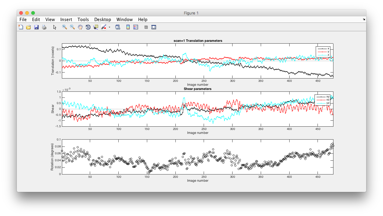
- Examine the motion correction matrices You can find these in plots → motion correction matrices. These show you how much the motion compensation algorithm had to move images.Does it show lots of movement? Do it on different scans. Are there any scans that might have so much head motion that you'd be suspicious of results?

Surfaces and flat-maps
It is often helpful to examine our data on renderings of the cortical surface. This is done by processing a high-resolution T1 image of the brain to find the borders between the gray and white matter and the surface of the brain. Then you can segment out just the cortical surface. This is useful since you can throw out data from outside the brain, or within the white matter and visualize on the cortical topography. FreeSurfer is a useful set of tools that can do this automatically on a T1 image (you type one command and then come back in 24 hours or so and it has segmented the brain and made triangulated surfaces. Check here if you wish to know more about surfaces and flat maps. In this section we'll take a look at surfaces and make some flat maps for visualization.
Alignment
Let's check the alignment between our anatomical and EPI scans. Typically, alignment is done to align scans done on different days (because your head is in a slightly different place in the magnet) - but, we also want to make sure that our anatomical scan lines up with our functional data.
We are going to use a tool called mrAlign to check the alignment between your T1 and your BOLD images.
- Remember subject ID Take note of the first four numbers in the mrLoadRet window title, s####. That is your subjectID.
- Quit mrTools File/Quit
- Run mrAlign From the Matlab command window type: mrAlign
- Load the canonical Go to File/Load Destination (volume). Navigate to ~/Desktop/sxxx/sxxx20250410/Anatomy/anat01_T1…(more stuff)….nii and load.
- Load the EPI Go to File/Load Source (inplanes). Navigate back to your data directory, but this time, instead of going into the anatomy folder, go to the “motion comp” folder and pick an image there.
- Examine alignment Move the slice slider at bottom to a slice in the center of the brain and adjust the alpha/overlay button until you can see both brains. Does the alignment look good? You can fiddle with the Translation and Rotation buttons to mess up the alignment and see what it looks like if it is not aligned.
We collected the scans during the same session, so they should be on top of each other! But, sometimes people move in the scanner - so it helps to perform an alignment.
Import surfaces
Ok. Now we are aligned to the canonical anatomy, we are ready to import a surface and take a look at it. You can skip these steps if the surface has already been imported, and instead select the surface or flat map in the Base dropdown menu, and then inspect the surface / flat map by going to plots/Surface Viewer or plots/Flat Viewer.
2025 note - we already imported the surfaces for you. So, you can skip the next part. Go ahead and change the “Base anatomy” to one of the surfaces - e.g. s0xxxAnat_left_GM. Then, go to plots → surface viewer. Select “whichSurface” as “3d anatomy”, and hit OK. This show you the same info you would get by walking through the steps below. Read through the following instructions, but you don't have to actually import anything.
- Go back to mrLoadRet Exit from mrAlign if you haven't already (File/Quit) and run mrLoadRet (type mrLoadRet in command window).
- Import surface Go to File/Anat DB/Import Surface from Anat DB. A dialog box will come up asking you to set the subjectID. Subject ID should show the same number as you noted above. Click Ok in the dialog box.
- Choose the left inflated surface From the surfaces folder load s####_left_Inf.off
- Choose the canonical In the next window open the s####.nii T1 file you used before.
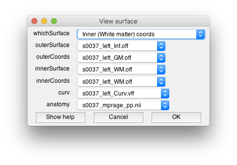
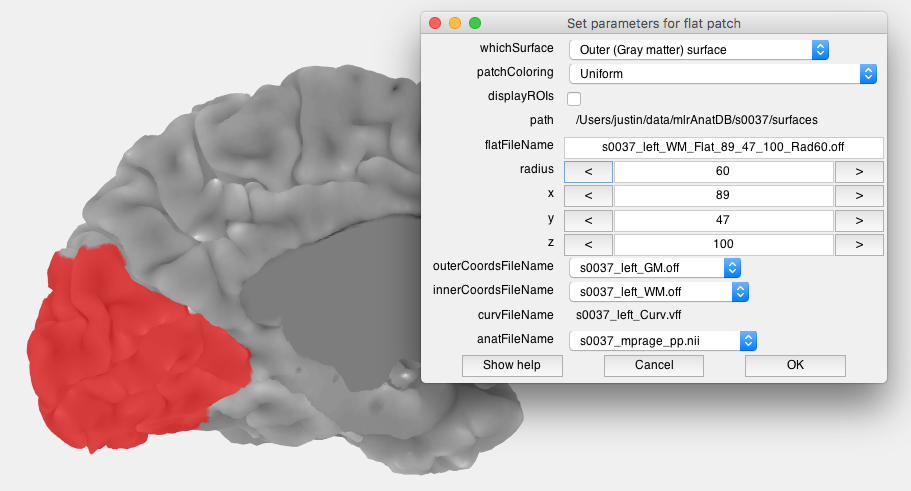
- Adjust surfaces Two windows should open, the “View surface” window allows you to set which surfaces you will view data on. There are two visualiation surfaces, outersurface and innerSurface. By having two surfaces, we can provide a slider later which will allow you to smoothly interpolate between the outer and inner surface for visualization. We will therefore use the inflated surface for the outer and the gray matter for the inner surface. The coords surfaces are really important. They determine where the data will come from that you visualize on these surfaces. You want to select the gray and white mater surfaces for these so that we can interpolate data from within the cortex. The dialog should look like the following when you are done (don't press OK yet!):
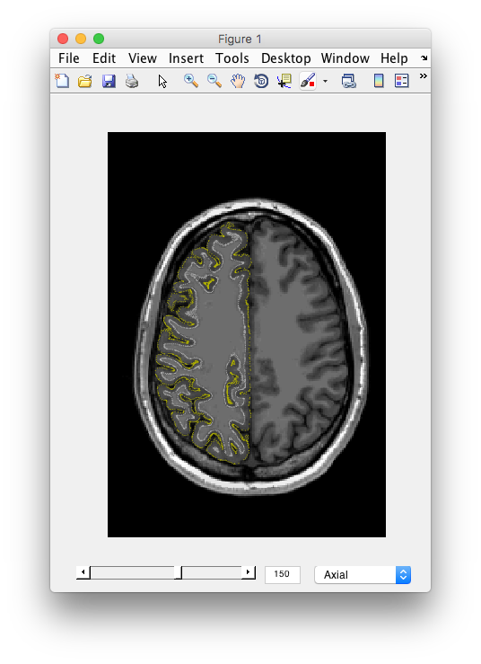
- Examine the segmentation Remember the segmentation should show you the outer and inner surfaces of cortex. Let's examine if the algorithm found it correctly. You should see the 3D anatomy in the other window with white and yellow dots. The white dots indicate the gray matter white matter boundary. The yellow dots indicate the pial surface, or the gray matter/CSF boundary. Scroll through the slices, do you see any errors? I.e. white matter that snuck in, gray matter that was left out, etc? Does the segmentation fail in any specific parts of the brain? How noisy does the gray matter and white matter look?
- Import and do other hemisphere If you are satisfied, click Ok to import the surface, and do the other hemisphere.


Make a flat patch
Often it is convenient to look at data on a flattened piece of cortex (makes it easier to view V1). Let's make flat patches around the calcarine sulcus. Again, if a flat patch is already made, then you can skip these steps and instead select the flat patch in the Base dropdown menu and inspect the Base by going to Plots/Flat Viewer.
- Rotate surface until you see the calcarine The calcarine should be easily visible on the medial surface of the occipital cortex. Make sure that Plots/Interrogate Overlay is not checked and rotate the brain around till you see the calcarine. You might also try moving the “cortical Depth” sliders on the top left. These will show you views from a fully inflated to the white matter surface.
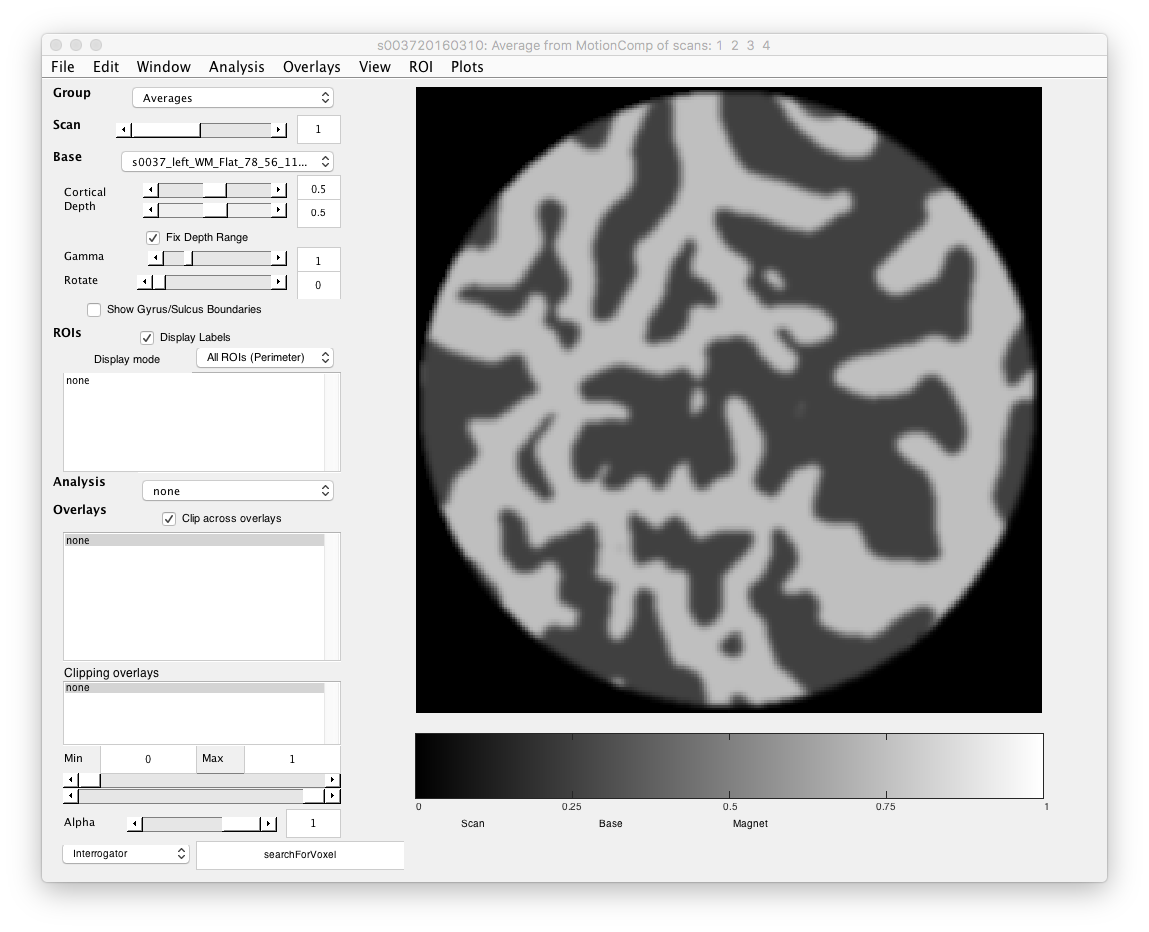
- Select the makeFlat interrogator Now, turn on interrogators (these are functions that get run when you click on parts of the brain). Go to Plots/Interrogate Overlay and select. In the bottom right, you should see an Interrogator drop-down. Select makeFlat.
- Click on the calcarine Now click on the calcarine near the occipital pole. This will set where you want to center your patch. You can play around with the radius until you get a patch that covers the whole calcarine (about 60 usually works)
- Run the flattening algorithm Click Ok. In the next dialog box use default options (flatRes=2, thershold checked and mrFlatMesh) and click ok. Check the command window, it will show you some updates as it is chugging along. You should now have a flat patch in the viewer
- Which way is up Most confusing thing about these patches, is which way is up? To figure this out
- Make sure session anatomy is loaded Peak in the Base drop-down and make sure you have the session anatomy anat… If you don't load it, and switch back to your flat map.
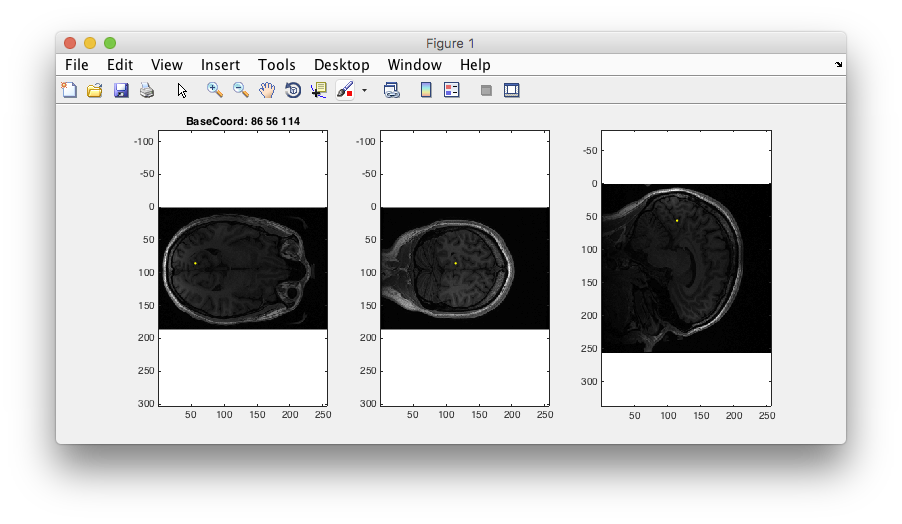
- Select searchForVoxel interrogator In the interrogator drop down at bottom left.
- Start search Click on any location in the flat patch. A dialog box should come up. Make sure that baseName is set to your session anatomy and that continuousMode is checked. We should have set this already for you - but doesn't hurt to double check.
- Find the top of the patch move your mouse (don't click) over the patch, you should see a yellow dot move around in the session anatomy noting the location where that part of the brain comes from.
- Click red close button Note that if you use ok, you will need to then wait a second - then you will need to set Base back to the flat patch (the searchForVoxel interrogator takes you to the location you clicked in the other anatomy.
- Rotate to top Now use the rotate slider at the left to rotate the patch until the location that you determined was at the top of the brain is at the top of the viewer.


You should do the above step - but we also give you pre-rotated flattops. You can import those by going to file, base anatomy, load, and picking lh_flat_rotated.img or rh_flat_rotated.img.
pRF analysis and V1 localization
Ok. Now we're ready to look at the pRF analysis.
- Averages Typically we average together a few scans where we showed the exact same set of bars to improve our SNR. This should already but done, so just switch to the Concatenation group (if it hasn't been done, just go to Analysis/Average Time Series and do it making sure that only the first 4 pRF scans have the include in average checked and click ok).
- pRF analysis The pRF analysis takes some time to run, so it should already be run for you. (If not, you would run it from the Analysis/pRF analysis menu).
- Examine r2 First thing to do is to see how much of the variance is accounted for. In the Overlays box at left, click on r2 to view the r2 overlay.Note that this example is from our regular pRF scans in which we run 8 runs and average which will give better SNR then the 4 runs that you ran.
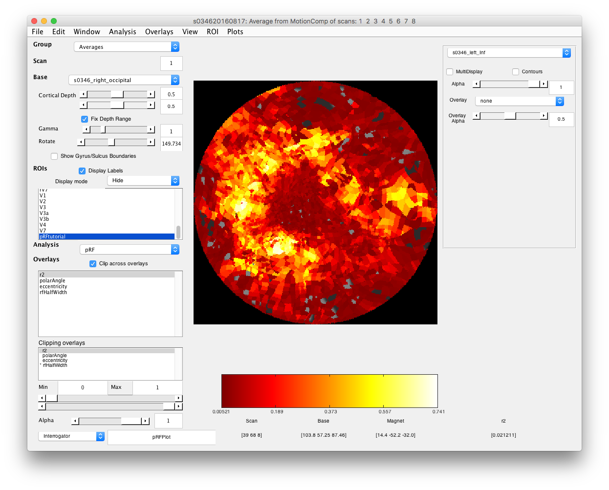
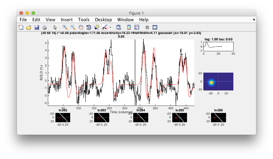
- Examine good voxel fits Making sure that the Interrogator is set to “pRFPlot” click on points in the flat map with high r2 (whitish). Does the fit (red) match the data (black)? If you move your mouse over the time series you should be able to see the stimulus and the receptive field at bottom that generated the model predictions. Makes sense?
- Examine poor voxel fits Click on a few voxels with low r2. What happened there? Why are the fits bad? Do they have visual responses?
- Select r2 cutoff voxels with poor r2 are just basically noise, so you may want to not view them in the overlays if it is easier. Set the Min slider at bottom left, making sure that “Clipping Overlays” is set to r2 to a value that gets rid of voxels with poor r2 (this can be pretty arbitrary for this purpose - if you really wanted to you could base clipping on some statistical test of goodness-of-fit.
- Examine eccentricity Chose “eccentricity” from the Overlays and examine that. Click on voxels to see if they match what is being displayed.
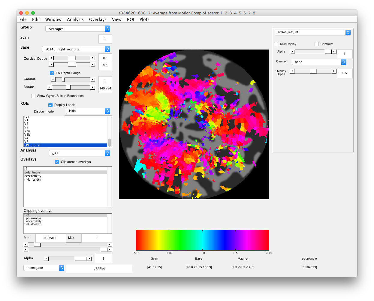
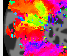
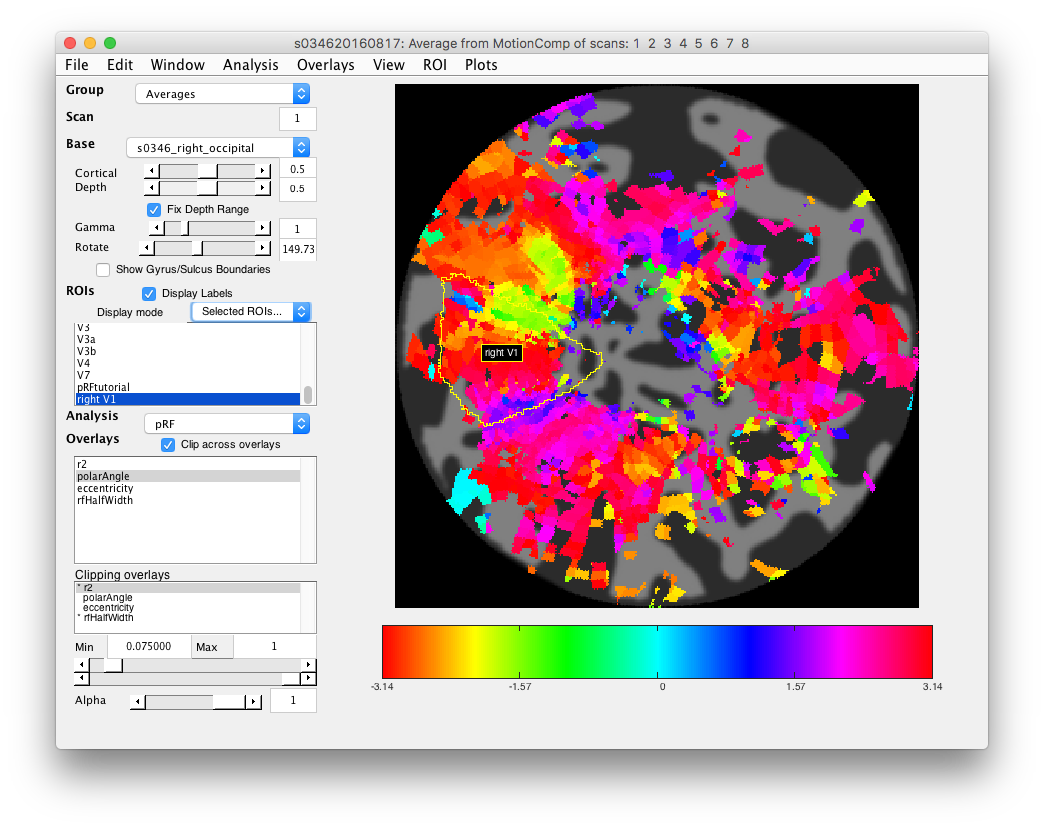
- Examine polar angle Choose “polarAngle” from the Overlays and examine that. This is how we are going to determine where V1 is. Remember that V1 is a full hemifield which is flipped on the cortex (goes from upper to lower visual meridian as you go from the bottom to the top of the calcarine sulcus). When you get to V2, the direction reverses and this is how you know where V1 is. In practice, you are going to look for colored stripes in the data where the vertical meridians are and draw an ROI around there for V1. You should look for two of the same color lower visual meridians (V1/V2 and V2/V3 borders, green in example below) in the top and two of the same color upper visual meridians in the bottom (magenta in the example below).Click a few voxels on these meridians to determine if the visual RFs are where you think they should be. Note that things may not look as pretty as in the above example, just because we collected less data. Ask if you can't figure out where V1 is!
- Draw V1 region of interest Turn off Plot/Interrogate Overlay. Go to ROI/Create/Polygon set the name to left/right V1 and click OK. Then on the flat map, draw your ROI by clicking. DOuble-click to finish the ROI.Make sure that Selected ROIs (Perimeter) is selected in the drop down at left for Display Mode and you should see your V1 ROI
- Draw V1 in other hemisphere Do the same for V1 in the other hemisphere.


It's easier to draw ROIs on the flat maps, but it is a little unintuitive to look at them there. Once you've drawn V1, go to ROI → convert → convert cortical depth, and hit ok. Select your ROI and hit OK again.
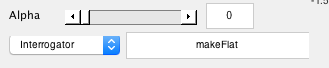
Then, go back to your left/right surface and find your ROI. Is it where you expected it to be? Hint - you might need to reduce the Alpha of your prf analysis in order to see it (bottom left of the window).
NEPR207 students - stop here! You made it!
Event-Related analysis
Now we will run an event-related analysis on your paradigm to see what you got!
- Concatenate scans together You will need to concatenate all the scans that you collected of your paradigm together. This should already be done. So just go to The Concatenation group. If not, you can run Analysis/Concatenate Time Series. Note that this high-pass filters the data at 0.01 Hz to remove low-frequency drift.
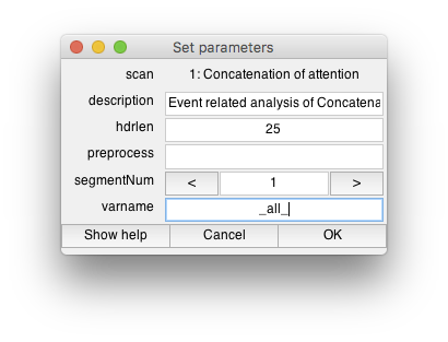
- Run evented-related analysis This should also already be run, but if not, you can go to Analysis/Event-related Analysis. Click Ok at the first dialog box and the second dialog box.On Set parameters dialog, you can choose the length of the hdr you want to calculate (the default should be fine). Also the name of the variable that you will use to run the deconvolution on (the variable may specify your attention or working memory conditions as different trial types and will be dependent on your particular paradigm). For now, let's just act as if all trials are the same and set varname to _all_Click Ok. This may take a few minutes to run - check the command window for progress.
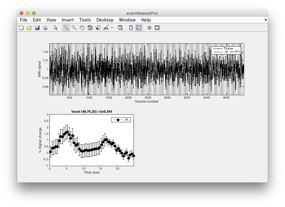
- Examine r2 You should see an r2 map, just like you did for the pRF. How much of the variance is being accounted for here?
- Select a high r2 voxel Click on one of the high r2 voxels (Make sure Plots/Interrogate Overlay) is on and the interrogator is set to eventRelatedPlot.


Next steps
- You might want to run an event-related analysis where you split out different conditions depending on your paradigm (ask one of us how to do that).
- Look in both hemispheres (switch to the other flat map).
- Look in different parts of the brain (switch the base back to the surfaces and look there).
- Look at the average response in V1 (click in the V1 ROI on event-related).
- Draw other ROIs and look at average responses.
- Run a classification analysis. To get the data see below
- Compute a contrast and display on the brain below.
- Examine your behavioral data. See below.
Make sure to save some figures (easiest is to do shift-command-4 then space and click on the viewer). These can be used for your presentation!
How to
Getting data from event-related analysis
You may want to get the data from the eventRelatedPlot so that you can do your own analysis. For example, replot the time series. Or, to run classification analysis using the region of interest you have define, like V1. To do that, click the “Save to Desktop” button in the eventRelated plot figure:

(eventRelatedPlot) Saving data from figure to variable eventRelated
>> eventRelated

eventRelated =

          d: [1x1 struct]
      voxel: [1x1 struct]
    stimvol: {1x3 cell}
        roi: [1x1 struct]
This has data from both the voxel and the region of interest (if you had clicked on an ROI). The fields in the data structure should be pretty straight-forward. For the voxel it looks like this:
- "matlab"
>> eventRelated.voxel

ans =

              vox: [61 64 15]
             time: [0.75 2.25 3.75 5.25 6.75 8.25 9.75 11.25 12.75 14.25 15.75 17.25 18.75 20.25 21.75 23.25 24.75]
             ehdr: [3x17 single]
          ehdrste: [3x17 single]
               r2: 0.3391862
          tSeries: [760x1 double]
    tSeriesByStim: {[19x17 double]  [17x17 double]  [18x17 double]}
Vox is where the voxel is in the data, ehdr contains the estimated hemodynamic response function for each condition (in this case 3 conditions) - i.e. your event-related analysis output for this voxel. ehdrste contains the standard error of those estimates computed over repetitions of the stimulus. r2 is the variance accounted for of the fit. tSeries contains the tSeries where this was computed from. tSeriesByStim is that same time series sorted by condition (i.e. in this case there were 3 conditions, with 19, 17 and 18 repetitions each of these 3 conditions. The tSeriesByStim has the time series broken up so that it contains the response from the start of each trial out for 17 volumes - the length of the computed event-related hdr). Note that these sorted tSeries do not deal with response overlaps - it's just the raw time series after each event. It also will contain nans in the time series for events which don't have complete data (i.e. the scan ended before the response was finished).
If you have a region of interest, it will contain similar fields, looking like this:
>> eventRelated.roi

ans =

               scm: [760x51 double]
            hdrlen: 17
              nhdr: 3
               dim: [2 2 2 760]
           volumes: [1x760 double]
              ehdr: [3x17 double]
           ehdrste: [3x17 double]
                r2: 0.60908429155102
              time: [0.75 2.25 3.75 5.25 6.75 8.25 9.75 11.25 12.75 14.25 15.75 17.25 18.75 20.25 21.75 23.25 24.75]
             covar: [51x51 double]
           roiName: 'lV4'
               roi: [1x1 struct]
    meanTimecourse: [1x760 double]
If you want the time series, it will be in the field roi:
>> eventRelated.roi.roi

ans =

             branchNum: []
                 color: 'black'
                coords: [4x636 double]
             createdBy: ''
    createdFromSession: 's037120180521'
         createdOnBase: 's0371_left_occipital'
                  date: '23-May-2018 16:26:13'
         displayOnBase: 's0371_left_occipital'
                  name: 'lV4'
                 notes: ''
             sformCode: 1
             subjectID: []
              viewType: 'Volume'
               vol2mag: [4x4 double]
               vol2tal: []
             voxelSize: [1 1 1]
                 xform: [4x4 double]
            scanCoords: [3x46 double]
               scanNum: 2
              groupNum: 4
              scan2roi: [4x4 double]
                     n: 46
               tSeries: [46x760 double]
         tSeriesByStim: {[19x46x17 double]  [17x46x17 double]  [18x46x17 double]}
Same format as the voxel, except you will see that tSeriesByStim has dimensions numRepeats x numVoxels x numTimePoints - where in this case the roi had 46 voxels.
Get behavioral data
If you want to analyze the behavioral data, you can get this from the workspace for the scan the mrLoadRet viewer is currently displaying (i.e. go to the group, scan in the GUI that you want the data for) and do the following:
>> stimfile = viewGet(getMLRView,'stimfile')

stimfile =

    [1x1 struct]    [1x1 struct]    [1x1 struct]
viewGet is a function that can get various things about the scan you are viewing (type viewGet without any arguments to see all the things it can get), getMLRView accesses the current view being displayed and stimfile are the files that we save about your experiment. Note that it returned an array of 3 of these for this particular experiment since there are 3 scans that were concatenated together, each having its own stimulus file. You can convert these into a format that is easier to parse by running getTaskParameters:
>> e = getTaskParameters(stimfile{1})

e =

                  nTrials: 20
              trialVolume: [1 14 26 39 53 69 85 100 113 129 145 160 175 191 206 220 235 251 267 NaN]
                trialTime: [1x20 double]
             trialTicknum: [1909 3078 4157 5326 6585 8024 9463 10812 11981 13420 14860 16210 17559 18998 20348 21607 22956 24392 25832 31319]
                   trials: [1x20 struct]
                 blockNum: [1 2 3 4 5 6 7 8 9 10 11 12 13 14 15 16 17 18 19 20]
            blockTrialNum: [1 1 1 1 1 1 1 1 1 1 1 1 1 1 1 1 1 1 1 1]
                 response: [1 1 1 1 2 1 1 1 1 2 2 1 1 1 2 2 1 1 1 NaN]
             reactionTime: [1x20 double]
    originalTaskParameter: [1x1 struct]
         originalRandVars: [1x1 struct]
           responseVolume: [10 23 35 48 62 78 94 109 122 138 154 169 184 200 215 229 244 260 276 NaN]
          responseTimeRaw: [1x20 double]
                 randVars: [1x1 struct]
                parameter: [1x1 struct]

>> e.parameter

ans =

    numJitter: [2 2 2 2 2 2 2 2 2 2 2 2 2 2 2 2 2 2 2 2]

>> e.randVars

ans =

                match: [1 1 1 1 0 1 1 1 1 1 0 0 0 0 0 0 1 1 0 0]
          orientation: {1x20 cell}
    orientationJitter: {1x20 cell}
      baseOrientation: {1x20 cell}
Note that variables that were used in your experiment will show up in either e.parameter or e.randVars depending on how they were coded. You can see the subject's response (which button was pressed) and what variables were set to as a function of trial. A nan would indicate no response. reactionTimes are in seconds relative to the beginning of the trial segment from which the subject could respond. Remember that if you want to compute something like percent correct, you probably want to do this by accumulating the data across all the scans (i.e. do a for loop over each stim file). To interpret the particular parameters and what constitutes a correct answer or not, consult with us about how your particular experiment was coded.
Displaying contrasts between conditions
You may want to display “contrasts” between conditions - i.e. color the brain according to which condition gave a larger response. One way to do that is to run a GLM and choose particular contrasts to display. It's point and click, but a bit involved because there are a lot of relevant settings. See here.
A simpler way is to compute something yourself and try to overlay it using the function mrDispOverlay. Here's a quick example, which takes your event related analysis and computes the difference in response for two conditions and displays that.
- Get event-related data Follow steps above to get the eventRelated structure.
- Compute difference for every voxel
% First get the estimated responses for all voxels out of the structure
ehdr = eventRelated.d.ehdr;
size(ehdr)

ans =

    92    92    54     3    17
The array is xDim x yDim x nSlices x nConditions x hdrlen in size (in this case a 92x92x54 epi image and 3 conditions computed for 17 time points). Let's just take the difference between the 1st and 2nd condition.
diff = nanmean(ehdr(:,:,:,1,:)-ehdr(:,:,:,2,:),5);
Note that I use nanmean since some timepoints will have nans in them if the motion comp has had to interpolate from outside the volume. Also, I'm just averaging across the whole response - you could try different things.
- Display in the current open viewer
mrDispOverlay(diff,2,'Concatenation',getMLRView);
Note that the 2 is for scan 2 and the group is 'Concatenation'. Once it is installed, it will show up in the viewer as the overlay mrDispOverlay.
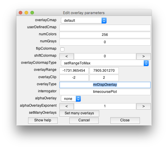
- Set overlay properties You may wish to choose how to display it (i.e. what colormap and so forth) by going to the menu item Edit/Overlay/Edit Overlay and choosing parameters. In particular, it may be helpful to set the clip boundaries - i.e so that only values within a range affect the display. I'll set these for this example to -2 and 2:And that looks like the following for this example: