Table of Contents
Signal detection simulation
We're going to simulate a signal detection experiment and an “ideal observer” (an observer who behaves exactly according to signal detection theory). This is always a useful thing to do when trying to understand a decision model, experimental method or an analysis tool. You get to control and play around with the simulation to see what effect it has on the analysis that comes out.
Signal detection is a general framework in which an observer tries to detect the presence or absence of a signal. What's a signal? Anything, really. Signal might be to detect a faint light (can you see whether a candle is lit in a window 1 mile away?). It could be to detect whether you see a friend's face within a crowd. Sometimes these experiments are called “Yes / No” experiments in that the observer has to say either “Yes” I saw it or “No” I did not. Sometimes there is a signal there (the candle was lit, your friend was in the crowd) and these are called signal present trials. Sometimes there is no signal there and those are called signal absent trials.
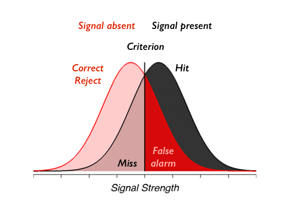
Subjects are right if the correctly detect a signal when it is present (hit) or when the correctly say the signal absent (correct reject). Similarly, subjects can make two kinds of mistakes - say that the signal was there when it was actually absent (false-alarm) or say that it was not there when it actually was (miss). These kinds of errors have completely unhelpful names in statistics (type 1 or alpha for false-alarm and type 2 or beta for miss), so its more helpful to think about them with these intuitive names!
A key idea that motivates the theory of signal detection is that you want to determine sensitivity (how good are subjects at detecting that faint candle light), but that there is an unaccounted for cognitive factor - what criteria the subject uses. A subject can have a very conservative criteria (only say the light is a candle if you are very sure). This will lower false-alarm rates, but then you may make more misses. A subject alternatively can change their criteria so that they are less prone to missing, but then they will make more false-alarms. Signal detection theory allows you to compute sensitivity and criteria separately from subject responses (i.e. the hit and false-alarm rates) so that you can determine how sensitive a subject is regardless of what arbitrary criteria they used.
For more background, check-out David Heeger's signal detection theory handouts.
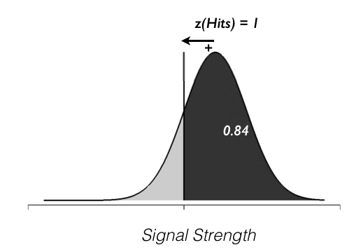
We will simulate a signal-detection experiment. On each trial, our observer sees an element sampled from either the signal present gaussian distribution or the signal absent distribution, which is also gaussian with the same standard deviation. The observer chooses to say “signal present” when the signal they see on that trial is above criterion and “signal absent” otherwise. The picture you should have in your head is this:
Make signalPresentAbsent array
So, here goes. First let's make a sequence of n=1000 trials in which 50% randomly are going to have “signal” and 50% are randomly going to have no signal. To do that we want to create an array called signalPresentAbsent that has 1's 50% of the time and 0's 50% of the time. For those of you who are familiar with matlab, go ahead and do this. If not open up the clues below:
Make signal array
Ok, now we want to simulate the signal that the observer actually gets to base the decision on. Remember that in applying signal detection to cognitive neuroscience you should be thinking of the signal as a neuron or population of neurons response and that the magnitude of this response (e.g. spikes per second) is monotonically related to the actual signal strength. The signal is corrupted by random noise. In particular, signal trials should come from some gaussian distribution and noise trials should come from another gaussian distribution that differ only in the means. This is an assumption about the process that is termed iid - the signal and noise come from independent identical distributions.
Ok, let's make a new array from our signalPresentAbsent array such that on signal present trials (i.e. when signalPresentAbsent == 1) values are picked from a gaussian distribution with standard deviation of 1 who's mean is 1 and on signal absent trails (i.e. when signalPresentAbsent == 0) values are picked from a gaussian distribution with standard deviation of 1 (that's the identical part of the iid assumption) but who's mean is 0.
Hint 1
Here are two ways that you can use the clue above. The first is perhaps conceptually easier, the second is a bit more efficient, but either will do.
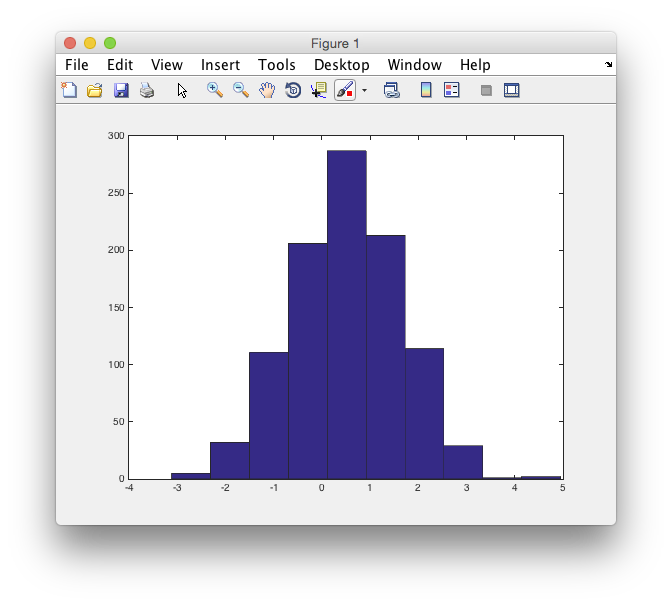
Let's take a look at the distribution of signal strengths we have created. You can do this by using the function hist
hist(signal)
It should look something like the following:
That's weird, it only has one peak, centered roughly around 0.5. Why? Shouldn't we have one peak at 0 and one peak at 1 for the signal present and absent trials? Yeah, but because they are so close together you can't really see them. You can see them separately if you display the histogram for just the signal present or just the signal absent trials. Try to do that.
Using that and the hist command you should be able to show the signal and absent distributions separately. Confirm visually that they have different means (signal present should be 1 and signal absent should be 0).
Now confirm numerically that the means and standard deviations are what they should be:
Hint 2
Ok, we're good to go. We have created the stimulus that our ideal observer will get to see (signal array) and we know which of the trials come from the signal and which from the absent distributions (signalPresentAbsent).
Make ideal observer responses
Now we are going to simulate an ideal observer which will behave just as signal detection says. They will choose signal present (response=1) when the signal they get to see (signal array from above) is greater than their internal criterion and they will choose signal absent (response=0) when the signal is below their internal criterion.
Let's start by making the criterion right in between the signal present and absent distributions that we created above. That is, let's set criterion=0.5 and make an array of responses. Try it yourself:
Solution 1
Calculate hits, misses, correct-rejects and false-alarms
Ok, so now we have our experiment (signalPresentAbsent) a simulation of the signal it generates in the observer (signal) and the ideal observers responses (response).
From these you should be able to calculate hits, misses, correct rejects and false alarms.
Do the proportions of hits, misses, false alarms and correct rejects make sense to you?
Calculate d'
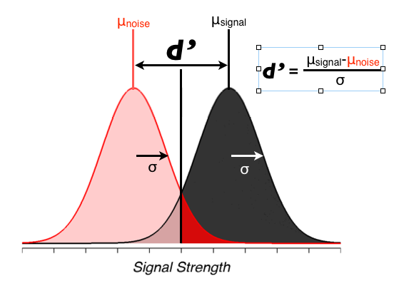
Now let's calculate d'. But, first a pop quiz: what should d' be given how we made the signal and noise distributions?
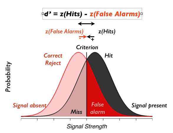
Ok, now we know what it should be, we're ready for pop quiz 2: what's the formula for computing d' from behavioral data?
Great. I knew you knew that.
So, how do we calculate those z's? If you know how to do it in Matlab, go ahead and do it and see if you get the expected d'. Otherwise use the hints.
How close is the dPrime you got to the expected value? Why is it different?
Different criterion
Now, simulate an observer that does not want to miss as much and see if you get a similar d' from their data.
You can try this for all sorts of criterion, is the d-prime measurement sensitive in any systematic way to the criterion?
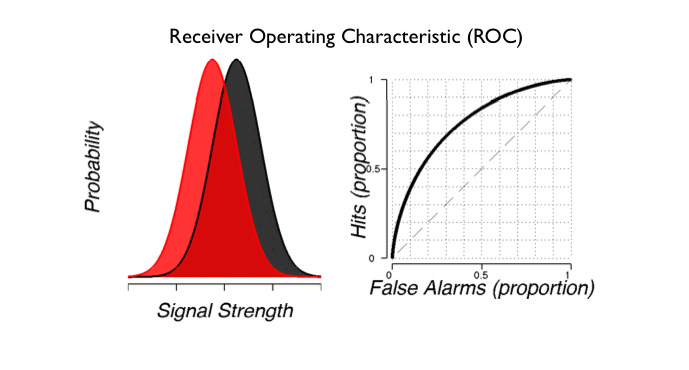
ROC calculation
Now, let's make an ROC curve. This assumes that we have some examples of samples from the signal and noise distributions. In the Newsome experiments these are the values of the spike counts for the neurons preferred direction (signal) and the neurons anti-preferred direction (noise, what they called the anti-neuron). Will just do it by pulling actual values from a signal distribution that is gaussian with mean of 1 and standard deviation of 1, just like we did above. For the noise, let's do mean of 0 and standard deviation of 1. Make two arrays of length n=1000, one for signal and noise using the techniques from above:
Check that the procedure worked by computing the means and standard deviations of signal and noise and making sure that they are what you expected (always good to double check everything when programming to make sure that things are working out the way you expected).
Ok, how do we compute the ROC curve? What's on those two axes. Remember?
Ok, so that is computed for various criterions, right? So, if you think you know how, try to compute a curve from the signal and noise distributions.
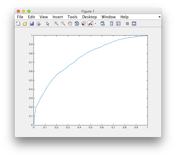
Ok, now plot it and you should get something like the following:
plot(falseAlarms,hits);
And, remember that the area under the ROC is performance on a two alternative forced choice task (2AFC). So, calculate the area under the curve and see what you get.
What did you get? Is it right? Well, one way to check is to see if a simulation of 2AFC will give you the same (or numerically similar) values. The experimental logic says that if signal is greater than noise then the ideal observer will get the 2AFC right, otherwise the observer will choose the noise interval and get it wrong. So, that's pretty easy to simulate. Try it!
Ratings experiment
When running a signal detection task you get one point on an ROC curve (hits vs false-alarms) from the data you collect, so you have to infer the rest of the curve based on the assumption that the underlying distributions are gaussian with equal variance. What if you don't want to do that, but you actually want to construct a full ROC from subject's data? What would you do?
Well, one way is to ask the subject to do the task several times each time asking them to either make sure they don't make too many false-alarms (and not to worry too much about misses) or vice-versa. That is, ask them to cognitively change their criterion.
A, perhaps, better way is to do a ratings experiment. Instead of asking subjects to say yes/no or present/absent, you ask them to rate, say on a scale of 1 to 5 the trial where 1 = sure that the target was absent and 5 = sure that the target was present. Let's see how that can give you a full ROC. First let's simulate that.
Ok, now we have the ratings of our ideal observer, how do we compute the ROC? Well, the trick is to take each rating as a different setting of the subject's criterion. Rating of 5 or better is a criterion that has very few false-alarms. Rating of 4 or better has more false-alarms and so on. In other words, you can compute your hits and false-alarm rates as a function of what the rating was. Try it out.
Look at your hits and false alarms. Do they make sense? As you go to lower and lower ratings, you should get higher numbers of hits, but also higher number of false-alarms.
Now just plot hits vs false-alarms and, voila, an ROC curve.
Challenges
Try running a simulation in which the standard deviation of signal and noise are not the same. What kind of ROC do you get from that? Is the standard calculation for d' still meaningful? What about the area under the ROC?
