Table of Contents
GLM statistics in mrTools
This wiki page provides some more background about the v2.0 implementation of the GLM code by Julien Besle (julienbesle@gmail.com) done at Nottingham, as well as a complete documentation of all parameters. For the original version of the GLM analysis, on which some of the code was based, see original GLM analysis.
In addition, you may want to read through other introductions to the GLM model, eg at the FMRIB in Oxford http://fsl.fmrib.ox.ac.uk/fsl/feat5/ or the online textbook at statsoft.
There is also a step-by-step tutorial on this version of the GLM analysis.
A quick primer on the General Linear Model
The goal of the General Linear Model (GLM)1) analysis is to explain an fMRI timeseries at a given voxel with a limited set of explanatory variables (EVs), sometimes also called regressors. EVs are physiological or experimental variables 2) with a known temporal structure, but unknown amplitude. For example a sensory stimulation in an fMRI experiment has a known temporal structure but we don't know how much it contributes to the fMRI variation with time. The goal of the analysis is to find out how much each EV contributes to the time-series.
The GLM model makes the simplistic assumption that the fMRI time-series Y(t) at a given voxel can be expressed as a linear combination of p known time-series X1(t),..,Xn(t) or EVs 3):
where β1,…,βp are real values called beta weights or beta estimates and ε(t) is a noise term that we are not able to explain 4). Beta estimates β1,…,βp represent how much each EV contributes to the fMRI signal Y(t).
This model is often denoted in matrix notation:
Where Y is a column vector of n recorded fMRI time-samples, β is a row vector of p estimates, X is the design matrix, i.e. a matrix of size n×p where each column represents an EV and ε is column vector of n random values. The goal of the GLM analysis is to find the values of the p beta weights that best explain the fMRI time-series, i.e. maximize the contribution of EVs (explained variance) and minimize the contribution of noise (unexplained variance) in the model.
The most common method to estimate these β weights is called Ordinary Least Squares (OLS). There are at least two conditions required to use OLS estimation:
- The assumption that the noise has no temporal structure (meaning that at each time point the level of noise is independent from the level of noise at other time-points)
- The condition that EVs are temporally independent from each other
Under these conditions, it can be shown that there is a unique set of beta weights that minimizes the contribution of the noise and that they are computed as
The requirement for independent EVs can be understood intuitively: if some EVs were not independent (i.e. if they had similar temporal structure, or one was a linear combination of other EVs), then it would be impossible to decide which EV contributes to a particular temporal structure in the data because there would be an infinite number of linear combinations that “best” explain the time-series. In other words, the design matrix in this case would be ambiguous. This would happen if two stimuli are always presented together: it is impossible to decide which or how much each contributes to the recorded fMRI signal.
Note that in the GLM analysis, each voxel time-series is analysed independently from the other voxels. There is no attempt to include a spatial structure in the model.
HRF models
It is well known that the hemodynamic response to an infinitely/very short stimulus (aka hemodynamic response function or HRF) is not a very/infinitely short increase in the fMRI signal. The signal variation following a sensory stimulation has a certain shape and a certain delay. and these temporal characteristics have to be taken into account in the GLM in order to obtain a better fit of the model with the data. This is done by convolving the design matrix, i.e. each EV of the model, with a model of the HRF to obtain a new model that reflects the variation of the fMRI signal rather than the variation of the experimental design.
Three models are currently implemented:
- A double Gamma function model: This models the HDR as a difference of 2 gamma distribution functions with three parameters:
- Shape of the positive Gamma distribution function (determines the peak latency of the HRF: panel A)
- Shape of the negative Gamma distribution function (determines the undershoot latency of the HRF: panel B)
- Scaling ratio of the postivie to negative gamma components (see panel D)
Because the parameters are fixed for all voxels, this model cannot accomodate HRF variations in delay across voxels (or conditions or subjects). However, there is an option to add the temporal derivative of the double gamma function as an additional component to the EV. Each EV is convolved not only with the HRF, but also its orthogonalized temporal derivative. This in effect doubles the number of EVs (the number of columns in the design matrix). Fitting the GLM for this design matrix produces 2 beta values per EV (columns in your original design matrix). Computing a linear combination of columns of the HRF model using a set of 2 beta values as weights would give you the estimated shape of the HRF for this EV.
- Basis set. The HRF is modeled using a number of independent components (3 or more ) or vectors that span a plausible space of shapes for the HRF.
In this case each EV is convolved with as many components as there are in the HRF model, resulting in a design matrix with (number of HRF components × number of EVs) columns. Fitting the GLM for this design matrix would produce (number of EVs) sets of (number of HRF components) beta estimates. Again, computing a linear combination of columns of the HRF model using a set of (number of HRF components) beta values as weights would give you the estimated shape of the HRF for this EV.
HRF basis sets must be constructed using FSL's Linear Optimal Basis Set (FLOBS). The default is to use their default 3-component basis set.
- Deconvolution: This is a special case where there is no attempt to explicitly model the HRF.
Rather, as many dimensions as necessary are provided in the HRF “model”, in order to capture/estimate the shape of the HRF on a given number of TRs. In effect the HRF model in this case consists of an identity matrix whose size defines how many TRs you want to estimate the HRF on. If for example you wanted to estimate the HRF for a 20 s period and your TR is 2s, you would use a 10×10 identity matrix. Each EV in your model would be convolved with this identity matrix to produce a design matrix with (10×number of EVs) columns. Fitting the GLM in this case would produce (number of EVs) sets of 10 beta values which would each have the shape of the HRF in response to each EV. Again, computing a linear combination of columns of the HRF model (the 10×10 identity matrix) using a set of 10 beta values as weights would give you the estimated shape of the HRF for this EV.
This is equivalent to running the event-related analysis in mrTools, but allows for statistical analysis (for example an F-test on a subset of beta estimates at different time points).
Statistics in the GLM
Descriptive statistics in mrTools currently consist solely of the coefficient of determination R2 which measures how well the model explains the variance in the timeseries.
Inference tests are based on the analysis of variance of the EVs of interest and residual noise.
All statistics (at least implicitly) require the computation of an estimation of the noise, aka residuals.
The estimated noise is the difference between the actual timeseries Y and the model Xβ
Coefficient of determination
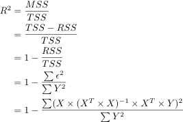
The coefficient of determination R2 is the ratio of the variance explained by the model to the total variance of the data
Where
- TSS is the total variance or total sum of squares, and is computed as the sum of the squared time-series values.
- RSS is the residual variance or residual sum of squares, and is computed as the sum of the squared residual values.
- MSS is the variance explained by the model or model sum of squares
The R2 value will be close to 0 if the time-series is dominated by noise and closer to 1 is the model explains the time-series. Note that R2 also depends on the number of independent EVs in the model: the more EV the higher the value, so while R2 values are useful to compare voxels that are analysed with the same model, they shouldn't be used to compare model fits with different numbers of EVs.
Inference Tests
Contrasts and T-tests
Contrasts are linear combinations of EVs that are of particular interest. They can consist in a single EV or a difference of EVs or a sum of EVs, etc… They are denoted as vectors of length p, where p is the total number of EV
Let's say you have 3 EVs in your model and you're interested in the contribution of EV1 to the hemodynamic response, the relevant contrast would be denoted:
C = [1 0 0]
If you wanted to look at the difference in contributions of EV2 and EV3 to the time-series, the relevant contrast would be or (one gives a value of opposite sign to the other). And your contrast value would be
Contrast = C×βT
Any contrast can be tested for significance using a T-test. T-tests return the probability that the contrast value is significantly different from 0 5) under the null hypothesis. The null hypothesis is the hypothesis that there is no effect, i.e. it describes the conditions under which the random distribution of contrasts (the null distribution) has a mean of 0. For parametric tests, we assume that the this null distribution is Gaussian with mean 0 and variance σ2.
T statistics are computed as:
where s2 is an estimate of σ2, computed as
Under the null hypothesis, T values follow a Student T distribution with (n-p-1) degrees of freedom. T-values can be converted to probability values or to a Z value (the value of the standard normal distribution that would return the same probability).
F-tests
This section is based on generalized hypothesis tests as described in Burock & Dale 2000
Contrary to T-tests, F-tests do not test whether a given contrast is significantly different from 0 but whether any contrast in a set of contrasts is significantly different from 0. F-tests are denoted as restriction matrices of size q×p (restriction matrix), where p is the total number of EVs and q<p is the number of contrasts in the set. Each row q in the restriction matrix therefore represents a contrast.
Let's say you have 3 EVs in your model and you're interested in the contribution of EV2 and EV3 to the hemodynamic response. If you only want to know whether any of those 2 EVs significantly contribute to the timeseries you could run an F-test that would be denoted
where the first contrast tests whether EV2 differs from 0 and the second contrast tests whether EV3 differs from 0. If it is significant, you will be able to conclude that either EV3 or EV3 contribute to the time-series, but you will not know which ones do (if you wanted to know, you would have to run 2 T-tests, one on each contrast, with the problem that you increase the number of statistical test performed and hence the family-wise error). Note that the current implementation requires the contrasts in a restriction matrix to be pairwise orthogonal (i.e. the dot-product of any pair of contrasts in the restriction matrix must be zero)
F statistics are computed as
Under the null hypothesis that none of the q contrasts significantly contribute to the timeseries, F follows a Fisher-Snedecor F distribution with (q,n-p) degrees of freedom. Like T-values, F-values can be converted to probability or Z values.
A simple example
The simplest example is if you wanted to test whether one of your stimuli evokes a significant hemodynamic response in a paradigm where there are, say, 3 different stimulations. Let's assume your paradigm has been designed so that your 3 stimulations are temporally independent. In this case you could have 3 EVs in your model, each one corresponding to each stimulation. After fitting the GLM, you would get 3 beta values that reflect how much each EV contributes to the time-series, or how much fMRI signal is evoked by each stimulus. If you only want to know whether stimulation 2 evokes a significant hemodynamic reponse, your contrast would be C = [0 1 0]
It is important to understand that even though you only want to look at one stimulus, your model still has to include all your stimuli. If you only used one EV, then the variance explained by the two other EVs would go either in the noise, decreasing the sensitivity or worse in the estimation of EV2, which would result in an increased likelihood of false positives.
Along the same lines, it is important to include in the model all the known temporal structure in the data, even if it does not correspond to task/stimulation. (Unfortunately, it is not currently possible to add nuisance EVs that cannot be represented as boxcar events convolved with an HRF model. Commonly modeled nuisance factors like low frequency drift and DC offset are removed by high-pass filtering and de-meaning respectively).
You might also want to test whether there is any effect of the stimulus type on the amplitude of the fMRI response. For this, you need to set an F-test that evaluates the probability that all pairwise differences between your 3 EV estimates are due to chance (main effect F-test). If you can reject the null hypothesis, then at least one pair-wise difference must be significantly different from 0. Because pair-wise difference contrasts (for example [1 -1 0] and [0 1 -1]) are not orthogonal, we cannot set the F-test restriction matrix as
Instead, we need to change our model in order to be able to express the main effect F-test with orthogonal contrasts. Instead of using 1 EV per stimulus condition, we are going to model our experimental paradigm with one EV representing the common BOLD response to any stimulation and 2 EVs representing any effect due to the fact that the BOLD response to stim 2 and stim 3 might differ from the BOLD response to stim 1. That is, the EV1 would model an HDR each time any of the 3 stimuli is presented, EV2 would model an HDR each time stim 2 is presented and EV3 would model an HDR each time stim 3 is presented.
In this new model, if we want to test for the existence of any difference between stim 1 and stim2 or between stim 1 and 3 (and as a consequence between stim 2 and 3), we only need to test the significance of EV2 and EV3. The restriction for this F-test will thus be:
which is a set of two orthogonal contrasts.
Correction for noise covariance
OLS estimation assumes that data points are temporally independent. In other words, timeseries are treated as random samples, ignoring any dependency between time-points. Since EVs are known (they aren't random variables), this is the same as saying that we consider the noise/residuals to be a sample of n values randomly and independently taken from a given distribution (Gaussian for all parametric statistical purposes)
But in fact, fMRI data are temporally correlated, i.e. two data points acquired in close temporal proximity are more likely to be alike than points that are acquired at two completely different times. Since the model does not include temporal correlation (although some of the temporal structure is modeled by convolving the time-series with a smooth HRF model), this is equivalent to saying that the noise actually has a temporal structure. The violation of the noise temporal independence assumption does not result in a biased estimation of the beta weights, but in a biased estimation of the residuals (they are over or underestimated). This in turn leads to biases in statistical tests (potentially a higher rate of false positives than the nominal 5% rate).
Several methods have been proposed to correct for noise correlation. Most are based on modelling the temporal structure of the noise by estimating the covariance matrix from the residuals (after OLS estimation) and including the covariance matrix in the computation of a new least square estimation.
Implemented methods include
- Covariance Correction Woolrich et al. 2001
- Generalized Least-Squares (GLS) Burock & Dale 2000, Wicker & Fonlupt 2003
- Pre-Whitening Woolrich et al. 2001
- Generalized Least-Squares Burock & Dale 2000, Wicker & Fonlupt 2003
Pre-whitening and GLS are mathematically equivalent and will produce the same results. My implementation of the GLS happens to be more computationally efficient, so I recommend using this one. It is the one I will describe in this section:
The first step is to get a description of the temporal structure of the noise. With a finite number n of data points, this can be described by an n×n noise covariance matrix. There are differents ways of getting this matrix. In the current implementation, the noise is approximated by the OLS residuals
Then we use single Tukey tapers Woolrich et al. 2001 to estimate the residual covariance matrix Λ. This consists in estimating the cross-correlation of the time-series up to a lag of 10 and put those values from the diagonal to the 10th off-diagonal of an otherwise empty matrix. 6) To improve the robustness of this estimate, Λ is estimated for each voxel on a within slice square-window of parametrizable size around this voxel. I found that at 1.5 mm3 resolution, 30 mm was the size that reduced bias the most, see this document: example of a correlated noise bias analysis.
Once you got Λ, you can apply the GLS method:
In the same vein, residuals, variance estimates, T and F statistics can now be computed as
NB: If you replace Λ by an identity matrix of size n×n, you get the OLS equations
These methods are quite computationally demanding and increase the computing time to several hours. It is advisable to restrict the analysis to a subset of voxels by changing the analysisVolume parameter.
Testing multi-component EVs
If you use multi-component EVs (for example by using the double-gamma model with derivative, a basis functions set or deconvolution), contrasts and restriction matrices have to be expanded to accommodate the new number of EVs. I don't think this is an area that has been explored a lot (although I might be wrong), but I found some inspiration in Burock & Dale 2000 I also made a few arbitrary decisions while trying to stay general. Generalizing T-tests and F-tests can be done using generalized hypothesis testing as described in section on Inference Tests.
Two ways of combining components made sense to me, although there might be other ones:
You could decide that you want to test a linear combination of EV components for each T-test/F-test. In this case contrasts and restriction matrices keep the same number of rows, but each column is duplicated (number of components) times. These duplicate rows will be set to 0 or any real weight depending on whether and at which level you want this component to be included.
Mathematically the new contrast/restriction corresponds to a Kronecker tensor product of the original contrast/restriction with a component selection matrix D, which in this case is a row vector of length (number of components). For example, if you have 3 components and you chose to only test the first two, D would be
If your contrast is, say, C = [1 0 -1], then the expanded contrast would be
Note how the component selection matrix is multiplied by each element of the original contrast vector and substituted to it.
Similarly, if your restriction matrix is
The expanded restriction matrix would be
Or you could decide that you want to test whether F-tests or T-tests are significant for any component. In this case, each contrast, i.e. each row of the restriction matrix 7) will be duplicated (number of components) times. Because the new restriction matrix needs have (number of components × number of EVs) columns, each column (each EV) also needs to be duplicated (number of components) times, resulting in a (number of contrasts × number of components) × (number of EVs × number of component) restriction matrix.
Each (number of contrasts × number of component) submatrix will be replaced by the component selection matrix D, which is a diagonal matrix where number on the diagonal are set to 0 or any real weight depending on whether and at which level you want to included this component. Here again, this is equivalent to the Kronecker tensor product of the single-component contrast/restriction matrix with the component selection matrix D.
For example, if you have 3 components and choose to test whether contrast C = [1 0 -1] is significant for any of the first 2 EV components, D would be
And the expanded contrast would be
Note that in this case, a contrast is replaced by a restriction matrix consisting of (number of components) contrasts. Therefore, one-sided T-tests cannot be performed, because the “contrast” has become an F-test and F-tests are two-sided.
If your restriction matrix is
the expanded restriction matrix would be
For the record, T and F statistics in the multicomponent case are computed as
An alternative way of testing multiple components would be to compute multivariate statistics using the components as the vector or multivariate random variable. This is yet to be implemented.
Scale of beta weights and conversion to percent signal change
Expressing beta estimates in terms of percent signal change seems to be a delicate problem. (Although percent signal change in itself is not an extremely meaningful measure, so I don't think there's anything to worry about.)
Let's assume that we converted the time-series to percent-signal change and that the mean of each time-series is zero. The problem stems from the fact that the scale of beta weight depends on the scale of the regressors (EVs). But what is the right scale for an EV? Assuming your design matrix accurately reflects the input to the hemodynamic response function, the scale of beta weights depends on the scale of the HRF model. So what should this scale be ? What size of the HRF model corresponds to 1% signal change in the time series ?
A further complication is that this also depends on the shape of the HRF and by the number of HRF components. Indeed, how to scale the different components relative to each other ?
This implementation of the GLM takes a pragmatic approach: the goal was that when you display the modeled response of a voxel using any HRF model, it should give you similar scaling, including when using the deconvolution HRF model.
Each component of the deconvolution HRF model models each time sample following a stimulus with a single 1. Therefore each beta weight (each time-sample of the estimated evoked response) is naturally scaled to the amplitude of the time-series. This is an appealing way of scaling beta weights, and is considered here the right scale for percent signal change.
If you consider the deconvolution HRF model (an identity matrix of size duration in TRs of the estimated response), each column has an integral of one and columns have the same norm. Setting the integral of each component to one guarantees that the scaling of the design matrix is conserved through convolution with the HRF model and therefore that the scaling factor between the matrix design and the time-series does not change. The equality of norms guarantees that all components participate equally to the estimated response. Provided that they are independent and in the absence of other information, this seems like the most reasonable assumption.
I extended this to other HRF models: after constructing the HRF model, the norm of all the components are equated. Then the matrix is scaled as a whole so that the mean column's integral equals 1. This way, beta weights should be on the order of the percent signal change of the time-series.
(NB: everything I just said about scaling might not apply in some special situations where the acquisition time is shorter than the frame period, such as sparse sampling. This needs more testing.)
Super-sampling and sub-sample estimation
Design supersampling
So far, we have assumed that EVs can only be defined at the temporal resolution of fMRI acquisition. But it could be the case that stimulations are defined at a higher temporal resolution, either because the stimulus duration is not a multiple of the volume acquisition time, or acquisition period (often improperly called TR) or because stimuli onset occur outside volume acquisition times.
In the current implementation, the user can either choose an arbitrary supersampling factor or let the software automatically set the minimal supersampling factor such that the smallest sub-acquisition onset time or stimulus duration can be resolved (down to a minimum of 50 ms). For example, if the stimulus duration is 1.6 s and the TR 2.4s, the supersampling factor is 3, because duration = 2/3 TR. Both the experimental design and the HRF model are constructed at the supersampled resolution and convolved into the design matrix. The design matrix is then downsampled at the acquisition rate.
Supersampling is done in such a way that the integral of the HRF corresponding to the duration of one TR is still 1, so that supersampling does not influence the value of beta weights.
On the other hand, it also sometimes happens that your stimulus times are slightly off TR, because of timing errors in the stimulus delivery program. In this case, you might want to force the stimulus onset to fall on the closest acquisiton or on the closest subdivision thereof by manually setting the supersampling to 1 or an integer value greater than one.
In most cases, changing the design supersampling will not change the result much because of the sluggishness of the HDR and will not result in sub-acquisition rate resolution of the HDR
Sub-sample estimation
In some special cases where the experiment has been designed for this purpose (stimuli are presented in a sub-acquisition rate fashion) , sub-TR resolution of the HRF estimation can be achieved using the deconvolution HRF model. For example, you might want to estimate the HDR every seconds when in fact the frame period is 2s.
This estimation supersampling is independent from the design matrix supersampling described above (although the latter is required to achieve sub-acquistion estimation).
Non-parametric Resampling tests
Resampling tests are based on the idea that the Null distribution can be estimated by resampling the data in an appropriate way instead of modeling theoretical null distributions using parametric functions such as T or F. Although computing-intensive, these methods allow to get rid of some assumptions on the distribution of noise (like normality)
There are at least two ways of resampling the data
- bootstrapping
- (re-)randomization (permutation)
In both cases, it is important to note that only the normality assumption can be dropped, not that of independence of the datapoints. This assumption plays out differently in the two cases
Most of what is said here comes from Westfall and S.S. Young, Resampling-based multiple testing: examples and methods for P-value adjustment (Wiley-Interscience, 1993).
Bootstrap Statistics
Bootstrapping is implemented in the case of the GLM as residuals bootstrapping, in which the Null distribution is approximated by resampling the estimated residuals:
(1) First the GLM is fitted to the time-series in order to get the parameter and residual estimates, as well as the statistics T and/or F (actual T/F).
(2) Then residuals are resampled with replacement, that is, N residual values are drawn at random and with replacement from the pool of N residual values (N is the number of time samples). This constitutes a new time-series. The GLM is fitted to this new time-series, and new statistics (T or F) are computed. These statistics represent the value of T/F you would expect under the Null hypothesis.
(3) By repeating this resampling (step 2) a large number of times (typically between 1000 and 10000), one can see how the actual T/F statistic compares to the distribution of statistics under the Null hypothesis. The P-value for the bootstrap test is the number of bootstrap statistic that are larger than the actual statistic divided by the number of bootstraps.
That resampled residual values represent the time-series under the null hypothesis seems a bit counter-intuitive but can be explained easily. Indeed, if there was no effect of the experimental manipulation (stimuli) you would expect to only measure noise, which is what residuals estimate. In this case, all parameter estimates β would equal 0, and the GLM would be
Y = βX + ε = 0×X + ε = ε
Time-series under the null hypothesis can therefore be modeled by using only the residual values. Since residual values are centered around 0, the bootstrap null distribution will also be centered around 0.
If the null hypothesis is indeed true, the estimated β values will be small and the actual statistic should be well within the bootstrap distribution. The P value will be large and we won't be able to reject the Null hypothesis.
If, on the other hand, there is an effect of the stimulation, and this effect is large enough, actual statistics will far from 0 and the p value will be small.
Now we can explain why we resample with replacement:
Under the assumption that errors ε are temporally independent, at each time point, any residual value could have happened. Therefore, a good way of modelling this is to draw at random each residual value from the whole set of measured residuals.
We've already noted that the temporal independence assumption is false (see Correction for noise covariance), but residuals can be corrected for covariance by pre-whitening the data.
Permutation (Re-Randomization) Statistics
Re-randomization, although based on the same resampling principle, is quite different. Instead of resampling residuals, stimulus times are shuffled in order to model the Null hypothesis. This has two implications:
- the temporal structure of the noise is preserved, so that one does not have to worry too much about noise covariance
- the Null hypothesis can only be modeled if stimulus times can be shuffled in a way that simulates an absence of effect. Therefore, the scope of rerandomization tests is more restricted than that of bootstrap test and in the current implementation, it is limited to 1 to 1 comparisons between EVs.
(1) First the GLM is fitted to the time-series in order to get the parameter and residual estimates, as well as the statistics T and/or F (actual T/F).
(2) All stimulus times from the subset of EVs involved the effect of interest are pooled together. For each EV, the appropriate number of new stimulus times are drawn at random without replacement from this pool to fill each number of stimulus per EV.
(3) step 2 is performed a sufficient number of times to obtain a reliable distribution for the statistic (typically 1000-10000 times).
(4) Resamplings that give a statistical value larger (or smaller, depending on the type of test) than the actual statistic are counted and this number is divided by the number of randomizations performed. This gives the p-value for the test. P-values can then be transformed to Z-values.
It is easy to see why this procedure is restricted to some null hypotheses. For example it cannot be used to test whether a parameter estimate is significantly different from 0 because there would only be one EV involved and no other EV to exchange stimulus times with.
On the other hand, it is particularly well suited to test whether two estimates A and B differ from one another. Pooling stimulus times for A and B together adequately model the null hypothesis that A and B actually come from the same population.
More complicated contrasts or set of contrasts might be tractable but each situation has to be dealt with individually. For this reason, randomization tests are only implemented here for one to one comparison contrasts (of the [1 0 0 -1 0] type).
It remains to be seen whether there is any superiority of re-randomization over equivalent bootstrap tests in this case. I would maybe expect an improvement in sensitivity for randomization tests, provided reshuffling exactly matches the contrast. My advice would be to not use randomization tests unless you have a good reason to.
There also are differences in the interpretation of bootstrap tests compared to re-randomization tests, in particular regarding generalizability (see Westfall and Young, Resampling-based multiple testing, 1993, chapter 6, p174-177).
A note of caution about block designs: depending on how stimuli are coded, resampling might alter temporal correlations and result in a biased estimate of the null distribution: If only the onset and duration of each block is coded, it should be fine because whole blocks will be moved around during resampling and this will not break the temporal correlation within a block of stimuli. But if each TR of a block is coded as an event, then blocks will be broken and the temporal correlation will be less in the resampled data than it should be. This undoubtedly will result in a bias.
Multiple testing P-adjustment
Everything said so far applied to tests at only one voxel at a time. That is, for each voxel, statistical tests estimate the probability that the effect is due to chance. The more voxels are tested, the more this probability will increase across all tested voxels and at some point, the probability to get one or several positive tests among the tested voxels when the null hypothesis is true (false positives) will be almost a certainty.
The probability to get at least one false positive when M hypothesis tests are run is commonly referred to as the Familywise Error Rate (FWER).
The aim of multiple testing control procedures is to ensure that this FWER does not surpass a given threshold (usually 5%) on average.
An alternative type of control is to control the False Discovery Rate (FDR), which is the proportion of false positive among all rejected tests. In this case the procedure ensures that the FDR does not surpass a given threshold on average.
Three types of methods are implemented
- Bonferroni procedures control the FWER in the strong sense, without taking into account the dependence structure of the voxels.
- resampling-based adjustment (only for parametric tests) which control the FWER in the strong sense and take into account any dependency between voxels
- FDR control adjustment (FDR) control the FDR in the strong sense but the FWER only in the weak sense.
Strong FWE control means that FWE is controlled to stay under the chosen threshold whatever the truth of any tested hypotheses. That is, even if half the voxel have a true effect (i.e. the null hypothesis is false), the FWE is still controlled for the remaining voxels for which the null hypothesis holds.
Weak FWE control means that the FWE is only controlled when the null hypothesis holds at all voxels simultaneously. The benefit of using the FDR method however is that it is more powerful.
All methods are implemented in a P adjustment form, whereby P values are transformed to incorporate FWER/FDR control. That is, at each voxel, the p-value is increased (significance is decreased) to indicate the best FWER that can be achieved at this voxel. For example, in a volume of 1000 voxels, a voxel with p=.001 means that the effect has less than 0.1% probability of being due to chance even given that tests have been run on the other 999 voxels.
Bonferroni Procedures
The classical Bonferroni adjustment procedure consists in multiplying the raw p-values by the number of tests (voxels) performed. It controls the FWER in the strong sense for any dependence structure between voxels. Because it is so general, it is also very conservative in that it decreases the probably of observing any significant effect.
The basic Bonferroni procedure is called a single-step procedure because all p-values are corrected at once.
The power of the Bonferroni procedure can be slightly improved by considering voxels in a step-wise manner.
Stepwise Bonferroni procedures consist in ordering the tests/voxels according to their uncorrected p-values, considering them one by one and adjust the procedure depending on the remaining number of tests instead of the total. The idea is that once a null hypothesis as a given voxel has been accepted/rejected, the number of tests to consider is decreased by one and the next adjustment step can be made less conservative
Holm (1979) devised a step-down Bonferroni procedure in which tests are adjusted from the most to the least significant. The most significant test is adjusted by multiplying the raw-p value by the total number of tests M. If the null hypothesis is rejected (at a given threshold, usually .05),then there are only M-1 null hypotheses left to test. Therefore, the next raw p-value can be adjusted by multiplying by M-1 instead of M. The step-down procedure proceeds until a null hypothesis cannot be rejected or until there is only one voxel left, at which point the adjusted p-value equals the raw p-value (it is multiplied by one).
Hochberg (1988) devised a step-up procedure that is slightly more powerful since it starts by considering the least significant test. The raw p-value for this test is adjusted by multiplying by 1. If the null hypothesis is accepted, then the next raw p-value is multiplied by 2 and so on until the most significant raw p-value. The difference with the step-down procedure is that if at any point the adjusted p-value is significant (at a given threshold, usually .05) all the remaining tests (that are more significant) are also rejected.
Hommel (1988) devised a stage-wise procedure that is even more powerful than the Hochberg procedure.
For all of these tests, an adjusted p-value can be computed without setting a threshold in advance (see Wright 1992). Adjusted p-values at a given voxel represent the lowest threshold that would be necessary for the nul hypothesis to be rejected at this voxel
Resampling-based adjustment
Because fMRI signal is spatially correlated (adjacent voxels are more alike than distant ones), Bonferroni procedures, even step-wise, are likely to be too conservative. Indeed, if there is an effect at a given voxel, then it is more likely that there will also be an effect at an adjacent voxel. But in Bonferroni procedures, the probability of a false positive at a given voxel is considered to be independent from that at another voxel, so adjacent voxels will be corrected as if the outcome of the test at adjacent voxels were unknown
One way to take into account the correlation/dependence existing between voxels is to use resampling tests (see Westfall and S.S. Young, Resampling-based multiple testing: examples and methods for P-value adjustment. Wiley-Interscience, 1993).
In resampling-based FWER control, a global statistic (typically the maximum value of the statistic across voxels) is computed at each resampling (boostrap or permutation). This yields the probability distribution of the largest statistic value across all voxels under the null hypothesis. Then raw p-values at each voxel are compared to this null distribution in order to obtain adjusted p-values. If such an adjusted p-value is less than .05 at a given voxel, this means that the probability of such a high statistical value, given all other voxels and their dependence structure is only 5% under the null hypothesis.
This is the equivalent of the single-step Bonferroni procedure. There is also a resampling-based equivalent of the step-down and procedures, in which raw p-values are ordered, and the null distribution of the maximum statistic is estimated across less and less voxels as the significance decreases.
A resampling-based step-up procedure (Troendle, 1996) also exists but has not been implemented
Ge et al. (2003) introduced a method to compute resampled-based FWER adjusted P-values based on bootstrap p-values instead of parametric statistics However it seems so far that the number of bootstrap needed to achieve proper control of the FWER is very large. Furthermore, the method requires to either keep an array of size number of voxels*number of permutations in RAM (typically several Gb) or to recompute the statistic in a second resampling loop.
Note also that, even though the correlation structure of the noise is taken into account, the global statistic used does not necessarily capture the spatial structure of the effect. The implemented maximum statistic tends to favor large effect sizes even on an isolated voxel over robust but small effects spreading on large regions of the brain. Use of the Threshold-free Cluster Enhancement can increase sensitivity to such large clusters
Adaptive procedures and the estimation of the number of true null hypotheses
Another way to increase the sensitivity while preserving control of the FWER is to take into account the likely number of true null hypotheses.
All methods presented above assume that the null hypothesis is true at all voxels in order to control the FWER. But in most cases, it can be assumed with some confidence that the Null hypothesis should be rejected in some proportion of the voxels i.e. the null hypothese is true only for M0<M voxels. If we can estimate this number M0, then we can apply the FWER adjustment using M0 instead of M simultaneous multiple tests and increase the power of the test.
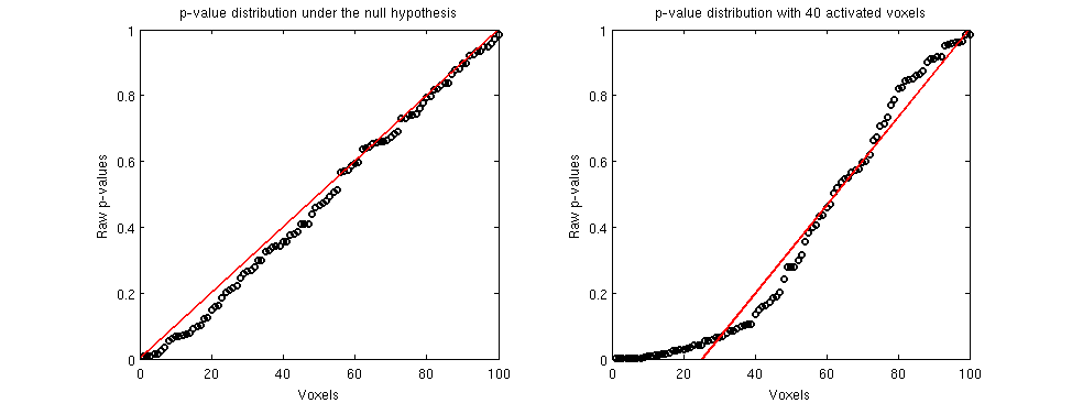
The general method to estimate M0 can be understood graphically by plotting the ordered raw p-value against their rank (quantile distribution) under the null hypothesis, p-values should be uniform and this plot should be linear (see left panel)
However, when some p-values do not come from the uniform distribution: there are more small P-values than expected. In the right panel of the figure, 40 of the 100 voxels are in fact activated and one can clearly see that the left part of the plot does not follow a straight line.
By fitting a straight line through the p-values that are believed to come from the null distribution, one can estimate the number of voxels where the null hypothesis is true (it is the inverse of the slope of the line). Ideally, we would like to estimate that there are 60 true null hypotheses in the right panel.
However random sampling has to accounted for and the crucial step in the procedure is to choose the number of tests on which the slope estimation should be based. In the figure, the number of the true null hypotheses is estimated to be 75 (instead of 60) using a least squares method.
Three methods are implemented to estimate M0, for single-step and step-down procedures, both Bonferroni and resample-based
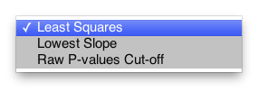
- a simple cut-off method in which the number of points chosen to estimate M0 depends on a fixed threshold
- the lowest slope method uses only two points (Hochberg & Benjamini,1990;Benjamini & Hochberg, 2000)
- a least squares method (Hsueh et al. 2003)
The lowest slope and least squares method are conservative enough to maintain protection of the FWER and the least squares method is apparently more powerful in the correlated case.
FDR control adjustment
Depending on the goal of the analysis, controlling the probability of getting even one significant voxel under the null hypothesis can be too stringent.
I has been proposed that, if the experimenter is ready to accept a small number of false positives, then controlling the proportion of false positives among the total number of tests performed (FDR) actually makes more sense (see Benjamini and Hochberg, 1995, Genovese et al., 2002).
In order to control the FDR at a given threshold, a simple step-up procedure on the ordered raw p-values can be used. In the adjustment version, raw p-values are multiplied by the number of tests performed (M) and divided by the number of tests that are more significant (K). Going from the least to the most significant voxel (unadjusted), the first adjusted P-values less than and given threshold (typically .05) is found and all voxels with a smaller unadjusted p-value.
This procedure controls the FDR whatever the truth of null hypotheses across voxels, under the assumption that voxels are independent or positively correlated. The independence assumption is clearly violated for fMRI data. However the positive correlation assumption might be reasonable (Genovese et al., 2002).
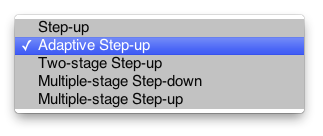
The step-up procedure can be refined by estimating the number of true null hypotheses in pretty much the same way as for FWER adjustment procedures (see Adaptive procedures and the estimation of the number of true null hypotheses). Other adaptive procedures have been proposed (Benjamini et al. 2006) and are implemented.
FWER vs FDR control
It is important to understand the difference of interpretation between an FDR and an FWER control procedures:
For FWER control procedure, if the assumptions are fulfilled, the expected proportion of cases where at least one non-activated voxel has an adjusted p-value of more than .05 is 5%. This means that if the procedure is run on 100 null data set, there should be no more than 5 datasets on average in which at least one voxel has an adjusted p-value of more than .05.
For FDR control procedures, if the assumptions are fulfilled, the expected proportion of non-activated voxels with an adjusted p-value of more than .05 is 5%. This means that if the procedure is run on 100 null data sets, for each dataset, there will be no more than 5 false positives on average. (Note that for a given dataset, if all null hypotheses are in fact true, the linear step-up FDR control procedure also controls the FWER.)
Obviously, FDR control procedures are more powerful. On the other hand, less can be said about particular voxels with FDR than FWER procedures. It has been argued that only procedures controlling the FWER in the strong sense allow to localize significant effects.
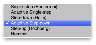
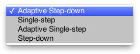
For a given type of control (FDR or FWER), the power will depend on the particular procedure used and on the distributional characteristics of the data. For any type of data, step-wise procedures are more powerful than single-step procedures and adaptive procedure are more powerful than non-adaptive procedure. In the current implementation, the default for FWER procedure is to use adaptive step-down procedures with least-square estimation of the number of null hypotheses.
Threshold-free Cluster Enhancement
Threshold-free Cluster Enhancement is a spatial filtering method that re-weights values in a 3D volume based on their spatial “area of support”. That is, not-so-large statistical values that are surrounded by not-so-large-values are increased in order to favor spatial cluster of lower values that might not otherwise be deemed significant.
It is called threshold free because, contrary to some other randomized-based techniques that are designed to detect cluster, it does not use statistical threshold to define the clusters.
TFCE is a non linear spatial filter, not an inferential statistical method in itself (it does output p-values). And since it transforms the value of the statistic at each voxel, parametric tests cannot be used to test the significance after transformation (although parametric statistics must be computed before application of the filter).
TFCE-transformed value have therefore to be tested using resampling tests (bootstrap or re-randomization). Basically, TFCE is applied to the T/F values computed in the volume of interest and resampling tests are used to compute non-corrected P-values at each voxel.
Because TFCE has to be applied to the whole volume of interest at once, each resampling must be performed on this volume. This limits the number of voxels that can be processed without using the virtual memory (depending on the available RAM). It is wise to not run whole-brain analyses using TFCE and to use a subset of voxel or ROIs instead.
Implementation of the GLM analysis in mrTools
Input and Output
Like other mrLoadRet analyses, the GLM analysis is performed on each scan of a group. If your data consists of different scans that you want to analyse as a whole, you will need to concatenate them beforehand. You will also need to link stim files to your scan.
The analysis results are output as an analysis structure that is installed in the group of the scans. This structure will contain all the computed beta, r2 values, as well as the analysis parameters. One overlay displaying the r2 values is also always output and installed in the view. In addition, the analysis can install one or several contrast, T-test and/or F-test overlays, depending on the chosen parameters.
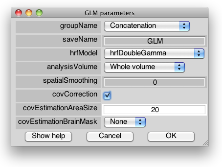
Parameters are input into successive parameter dialog boxes. Hitting the Cancel button re-opens the previous parameter dialog. To cancel all the parameter dialogs at once, press the close button at the top of the dialog window instead of the Cancel button.
The analysis can also be scripted (see Using the GLM analysis in a script).
Parameters
Analysis Parameters
groupName
Which group the data is taken from and the analysis is saved to
saveName
Name of the analysis to save
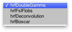
hrfModel
This specifies what function will be used to model the HDR impulse response (actually, the HDR corresponding to a stimulation of 1 TR, see Scale of beta weights and conversion to percent signal change).
Four functions are available, but you can write your own as long as it has the same input and output parameter. Both open a popup menu later where their parameters have to be specified
- hrfDoubleGamma: Models the HDR with a double gamma function, with three free parameters
- hrfDeconvolution: Just creates an identity matrix of the required length hdrlen (in s). This is equivalent to running the deconvolution analysis, but allows for statistical analysis (for example an F-test on a subset of time samples).
- hrfFslFlobs: models the HDR using any arbitrary basis functions set. The set has to be constructed first using FSL FLOBS
- hrfBoxCar: models the HRD with a simple boxcar function
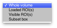
analysisVolume
This specifies on which voxels the analysis will be run. 'Whole volume' will analyze all the voxels of the scans. 'Subset box' will analyze a rectangular cuboid subset of the data. Coordinates of the cuboid will have to be specified in the scan-specific parameter dialog box. 'Loaded ROI(s)' will only analyze voxels in loaded ROI(s) and 'Visible ROI(s)' only in ROIs that are visible in the main mrLoadRetGUI.
Restricting the analysis to a small volume is important for noise covariance correction because it decreases the computation time and for randomisations on TFCE-transformed data, because Matlab must be able to hold the (number of voxels × number of randomzations) in memory. So if you have specific anatomical hypotheses, use this feature.
If noise covariance correction is on and the covariance matrix is estimated on an extended spatial window, voxels around the ROIs will automatically be loaded too. (Note that this is not the case for 'Subset box')
spatialSmoothing
If >0, spatially smoothes the time series with a gaussian kernel of width spatialSmotthing at half-maximum (expressed in voxels).
covCorrection
Whether you want to take into account the noise covariance in the GLM. This will not significantly change the estimates, but will generally produce more accurate statistical tests by reducing the bias in the estimation of the noise variance.
CovEstimationAreaSize
Size in voxels of the square window on which the residuals correlation matrix is estimated. I have found that the value that gives a false positive rate the closest to the nominal is 20 voxels at 1.5 mm resolution (30 mm), by running the tests on a resting state dataset (see Correction for noise covariance). But I haven't tested sensitivity (by looking at the power on a stimulation dataset).
covEstimationBrainMask
To estimate the noise covariance, it is best to restrict the covariance matrix estimation to brain voxels, i.e. excluding bone and extracranial voxels. If you specficy an ROI here, voxels outside this ROI will be excluded from the covariance matrix estimation.
HRF model menus
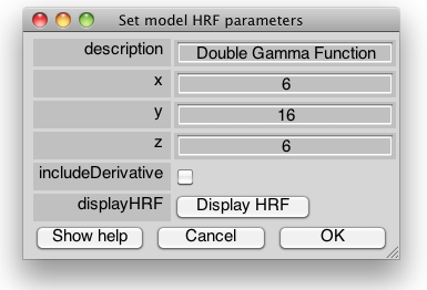
hrfDiffGamma
description
A string describing the model
x,y,z
Free parameters of the model: x=time to positive peak, y=time to negative peak, z = amplitude ratio of positive and negative peaks (see HRF models).
includeDerivative
if selected the model will consist of two components: the double-gamma and its orthogonalized derivative. The derivative allows to model changes in the HDR delay (changes in delays result in changes in the amplitude of the derivative, with positive values corresponding to an earlier peak).
displayHRF
Displays the HRF model sampled at the acquisition rate (NB: this does not include supersampling and acquisition time parameters because they are specified later).
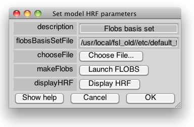
hrfFslFlobs
description
A string describing the model
flobsBasisSetFile
Text file output by FSL FLOBS that specifies the basis set. The default is the default FLOBS basis set.
chooseFile
This button will open a dialog to select and Basis Set file.
makeFlobs
This button will launch FSL FLOBS. You must have FSL installed to use this function.
displayHRF
Displays the HRF model sampled at the acquisition rate (NB: this does not include supersampling and acquisition time parameters because they are specified later).
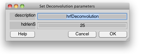
hrfDeconvolution
description
A string describing the model
hdrlenS
Duration of the HRF to be estimated in seconds. The number of samples estimated will depend on the frame acquisition rate and the estimation supersampling parameter.
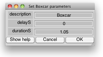
hrfBoxcar
description
A string describing the model
delayS
Delay between the stimulation event and the rising edge of the boxcar function.
durationS
Duration of the high state of the boxcar function.
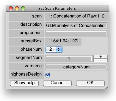
Scan-specific dialog menu
This menu will not appear if you are using non-MGL stimulus files, you have not chosen a subset box as the analysis volume and your file is either not concatenated or not high-pass-filtered
decription
A string describing the analysis.
preprocess
Path to a preprocessing function tha can be used to modify the stimulus timing. Preprocessing functions take the d structure as input and output.
subsetBox
Dimensions of the subset of voxels that will be analyzed (in scan coordinates). The matrix must be of the form [X1 X2;Y1 Y2;Z1 Z2], where X1 and X2 define the boundaries of the subset box in the X axis, Y1 and Y2 the boundaries in the Y axis, etc…
As of now, the size of the output overlay will be identical to processing the whole volume because non-computed values are just replaced by NaNs. NaNs do not take space on disk, but they do in memory.
taskNum
This parameter will only appear if you are using MGL stimulus files and your experiment has several tasks
phaseNum
Phase of the your experiment in which the stimuli of interest are presented. This parameter will only appear if you are using MGL stimulus files and your experiment has several phases
segmentNum
Trial segment in which stimuli are presented. This parameter will only appear if you are using MGL stimulus files and your experiment has several phases
varname
Name of the variable of interest in your MGL file. Press the help button to see the possible values. You can use a string that is combination of several variables here (see getStimvolFromVarname).
highpassDesign
If you're running an analysis on concatenated files that have been highpass-filtered, the design matrix should be filtered with the same filter. However you have the option to disable filtering of the design.
projectOutGlobalComponent
If you're running an analysis on concatenated files for which the mean time-series in an ROI has been projected out, the design matrix should be transformed the same way. However you have the option to disable this.
sameForNextScan
When setting the parameters for several scans in a group, uncheck this box if the parameters are different for different scans.
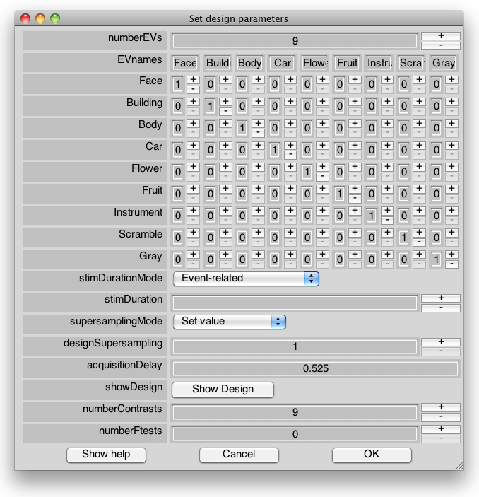
Design parameters menu
numberEVs
Number of Explanatory Variables (EV) in the model (Not including the number of components in the HRF model). This will normally correspond to the number of different stimuli in your experiment. However, in case your EVs consist of combinations or subsets of stimuli, you can add/remove EVs. To remove EVs, simply fill the correspongin columns with zeros. To add EVs, specify the desired number and press OK. This will re-draw the menu with the correct number of columns. You can choose 0 here if each EV exactly corresponds to each stimulus.
EVnames
Names of each Explanatory Variable to include in the model
EV definition vectors
Each line stands for a stimulus from the stimulus file(s) and each column defines an EV. For each EV, put 1 in the row(s) corresponding to the stimuli to include in the EV. These vectors form a matrix that transforms stimulus onset times into EV onset times.
stimDurationMode
How the duration of each stimulation event is determined. This is the duration of each stimulation or train of stimulations before convolution with the HRF model.
- Event-related: each stimulation event will be considered to last exactly one dynamic sca. Use this for event-related paradigms in which the effect of stimulus duration is not important. This is the default and only option for deconvolution models. If supersampling is used, the stimulus will be considered to last the duration of one sample in the supersampled model.
- Block: each stimulation will be considered to last until a different stimulus type is presented. Use this option for block design in which only the onset of the stimulus is specified. Note that this requires to have rest periods coded explicitly as events.
- Set value: uses the value specified in the next edit box.
- From file: this option will appear only if you're using stim files of the 'mylog' type that specify both the onset and duration of each stimulation event (see Event Related Analysis).
stimDuration
Duration of each stimulation event. This is only used if 'Set value' has been selected in the above dropdown list.
supersamplingMode
Whether and how to supersample the design matrix. If 'Set value' is selected, the design will be supersampled at the value specified in the edit box below. Use 1 if no supersampling is required (most cases). Stimulus onsets and duration will be rounded to multiples of the acquisition period divided by the supersampling factor. If 'Automatic' is selected, the design matrix will automatically be supersampled to accommodate stiumulus onsets and durations and acquisition durations that are not multiples of the frame period.
designSupersampling
This will only appear for non-deconvolution HRF models and specifies the supersampling factor if 'Set value' has been selected in the above dropdown list. Set this to more than one to make the model timing more accurate by taking into account sub-TR stimulus onsets/durations and acquisition durations.
estimationSupersampling
This will only appear if the deconvolution model has been selected. This parameter will set both the supersampling factor of the design matrix and the supersampling factor of the HRF deconvolution model. This allows to estimate the HRF shape beyond the acquisition rate, provided stimuli have been presented at different time intervals relative to the start of the acquisition.
acquisitionDelay
Specifies at what time during the frame period, the image is actually acquired. It should be set to the middle of the acquisition period, and will usually correspond to the middle of the frame period for continuous acquisition (the default), unless the acquisition time is shorter than the frame period (as in a sparse imaging sequence) or the time-series has been slice-time corrected to some specific time in the slice sequences. By default the acquisition duration is assumed to equal the frame period, unless acquisitionDuration is specified (see below). Example: For sparse acquisition with at TR of 7.5 s and an acquisition time of 1.5s at the start of the frame period, this should be set to 0.75, acquisitionDuration should be set to 1.5s (see below) and the design supersampling should be set to 7.5/1.5 = 5 (or superSampling mode set to 'Automatic'). Note that the acquisitionTime parameter is also taken into account when generating the double-gamma or FLOBS HRF models, such that the HRF model will be sampled at the specified acquisition time (and missing acquisition times for sparse acquisition) rather than at the centre of the frame period (or sub-samples).
acquisitionDuration
Duration of the data acquisition. This is set to the frame period by default, but should be changed to the actual acquisition duration if different from the frame period (e.g. sparse imaging or slice-timing corrected data).
showDesign
This will plot both the experimental design (i.e. after application of the stimulus-to-EV matrix,stimulus duration and supersampling) and the convolved design matrix (i.e. after convolution with the HRF model)
numberContrasts
Number of contrasts for which you want to create overlays and run a T-test. Contrasts are linear combinations of EVs that are of particular interest and that you want to display as a map. This will output at least 2 overlays for each contrast (the contrast value and its associated uncorrected T-test statistical map).
numberFtests
Number of F-tests. This will output at least one additional overlay per F-test (the uncorrected statistical map).
outputEstimatesAsOverlays
This will output the beta estimates as overlays (one per EV) without having to select the corresponding contrasts and associated statistics.
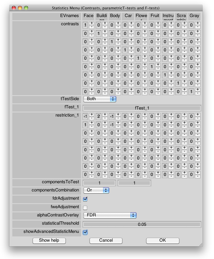
Contrasts and Statistics Parameter Menu
Contrasts
This appears only if you specified a number of contrasts >0 in the previous dialog menu. Each row of the contrast matrix stands for 1 contrast. Each column corresponds to an EV. Each row of the matrix thus specifies the weights of the EV in this contrast. It is good practice to test only for orthogonal contrasts, however there might be cases in which non-orthogonal contrasts are more sensible.
tTestSide
By default, contrasts are tested using a bilateral t-test. If you have an hypothesis on the sign of the contrast, you can choose left-sided (tests the hypothesis that contrast*betas <0) or right-sided tests (test the hypothesis that contrast*betas >0).
fTestName_#
This appears only if you specified a number of F-tests >0 in the previous dialog menu. Name of F-test number # (e.g. 'Main effect').
restriction_#
Restriction matrix for F-test number #. Each row stands for a contrast of the F-test and each column corresponds to an EV. Contrasts are linear combinations of EVs. There can be less contrasts than the number of lines (simply put all the row to 0 to remove a contrast) but there cannot be more than (number of EVs)-1 contrasts and contrasts have to be orthogonal.
These two last parameter entries will be repeated as many times as there are F-tests.
componentsToTest
For EV models with several components (several dimensions), specifies which component should be included in the test.
Example: You run a deconvolution analysis; the frame period is 2s; and you want to estimate the HDR for 25 s. In this case, the HRF model would have 13 components (25/2=13 frame periods). You can then specify an F-test such as: [0 1 1 1 0 0 0 0 0 0 0 0 0], which tests if any of the 2nd, 3rd an 4th time samples are significantly different from 0.
componentsCombination
For EV models with several components, specifies how the components are combined? Choose 'Add' to use the above vector as a linear combination of components in a single contrast, and 'Or' to include each non-zero component as an independent contrast in an F-test restriction matrix. Note that for Contrasts, option 'Or' will automatically turn the T-test into an F-test if more than one component are tested. Therefore one-sided T-tests are not permitted in this case.
fdrAdjustment
Whether to compute FDR control adjustments. The default is to use the adaptive step-up method with a least-square estimation of the number of true null hypotheses. These defaults can be modified in the advanced statistics menu.
This will output an additional overlay per contrast/F-test and per type of statistical test.
fweAdjustment
Whether to compute Bonferroni FWER control adjustments. The default is to use the adaptive step-down method with a least-square estimation of the number of true null hypotheses. These defaults can be modified in the advanced statistics menu.
This will output an additional overlay per contrast/F-test and per type of statistical test.
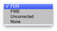
alphaContrastOverlay
statisticalThreshold
Threshold to apply to the statistical overlay, expressed as a P-value. Threshold will transformed to the appropriate Z or -log10(P) if these output have been selected (see advanced statistics menu). Overlays are not hard-thresholded and threshold can be modified after the analysis is run.
showAdvancedStatisticMenu
Check this box if you want to change the default method for FWER/FDR control, the default statistical output type, compute bootstrap confidecne intervals, etc…
Advanced Statistics Parameter Menu
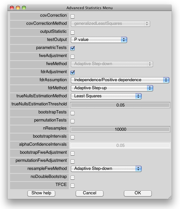
covCorrection
Whether you want to take into account the noise covariance in the GLM. This will not significantly change the estimates, but will generally produce more accurate statistical tests by reducing the bias in the estimation of the noise variance.
covCorrectionMethod
Covariance correction is slightly faster, but not as accurate as Generalized Least Squares. Pre-whitening is equivalent to Generalized Least Squares, but slower.
However, if bootstrap tests are used, pre-whitening is faster than Generalized Least Squares because the computationnally demanding calculations are done only once before boostrapping.
CovEstimationType
Method used for noise covariance matrix estimation. This feature has been disabled because only one option is currently implemented (Single Tukey Tapers).
Covariance matrix factorization
This feature has been disabled because only one type of factorization is implemented (Cholesky Factorization), but others are possible. Pre-whitening requires the computation of a matrix K such that K'K = Λ^-1. Since Pre-whitening gives the same result as the GLS, which doesn't (explicitly) use factorization, it's probably fine.
Correcting for non-linearity
This feature is still under development and has been disabled in the GUI. If Correction is selected, a forward correction based on Wager et al., 2003 is used: When convolving the HDR to the impulse matrix, a maximum value is imposed on the regressor, which saturates at a value proportional to the max amplitude of the model HDR used.
outputStatistic
Whether to ouput the test statistic value (T or F) in an overlay in addition to the normalized outcome of the statistical test (P/Z value)
testOutput
Type of statistic to output as an overlay for parametric/bootstrap/permutation tests: P values will output the probability value associated with the T or F statistics of a T-test/F-test. Z value will output the associated quantile of the standard normal distribution. -log10(P) value will output the opposite of the log transform of the P value. The default test output type can be set as an mrPreference using
mrSetPref('statisticalTestOutput','Z value').
parametricTests
Whether you want to perform parametric tests (the default). You might want to disable this if you're only interested in bootstrap/permutation tests and do not want to output an additional overlay per contrast/F-test
fweAdjustment
Whether to compute Bonferroni-type FWER control adjustments. Adjustments will be performed on parametric and/or bootstrap and/or permutation raw statistical maps.
fweMethod
fdrAdjustment
Whether to compute FDR control adjustments. Adjustments will be performed on parametric and/or bootstrap and/or permutation raw statistical maps.
fdrAssumption
Whether FDR adjustment are computed under the assumption that voxels are independent/positively corrected. Adjustment without assumption are only implemented for step-up and adaptive step-up and two-stage step-up procedures. The default is to make the assumption.
fdrMethod
trueNullsEstimationMethod
How the number of true null hypotheses is estimated for adaptive methods (see Adaptive procedures and the estimation of the number of true null hypotheses). The default is 'Least-squares'. This applies both to FWER and FDR adaptive adjustments
trueNullsEstimationThreshold
Raw p-value threshold for 'Raw P-value cut-off' method
bootstrapTests
Whether you want to perform bootstrap tests. This will output an additional overlay per contrast/F-test.
permutationTests
Whether you want to perform permutation tests. This will output an additional overlay per contrast/F-test.
nResamples
Number of resampling steps for bootstrap/permutation tests
bootstrapIntervals
Whether to compute residual bootstrap confidence interval for parameter/contrast estimates. This requires a lot of memory and should be run on partial volumes only.
alphaConfidenceInterval
Criterion value for the confidence interval. For example .05 would give you a .95 confidence interval around the parameter estimates.
boostrapFweAdjustment
Whether to compute bootstrap-based FWER control adjustments. Adjustments will be performed on parametric and/or bootstrap raw statistical maps. The default is to use the adaptive step-down method with a least-square estimation of the number of true null hypotheses.
This will output an additional overlay per contrast/F-test and per type of statistical test.
Bootstrap FWER adjustment for bootstrap statistics uses a double-permutation algorithm that requires a lot of memory and can be disabled (see 'noDoubleBootstrap').
permutationFweAdjustment
Whether to compute permutation-based FWER control adjustments. Adjustments will be performed only on parametric statistical maps. The default is to use the adaptive step-down method with a least-square estimation of the number of true null hypotheses.
This will output an additional overlay per contrast/F-test.
resampleFweMethod
noDoubleBootstrap
Check this if you don't want to run the resampled-base FWER control on bootstrap P-values, but only on parametric tests. Double bootstrapping requires a lot of memory in the current implementation.
TFCE
Whether you want to perform Threshold-free Cluster Enhancement before computing statistical maps. TFCE can only be used in conjunction with bootstrap/permutation tests or for resample-based FWE adjutment on parametric tests.
Note that currently, TFCE is performed using FSL. So you need to have FSL installed and to set the MR preference:
nrSetPref('fslPath','yourFSLpath')
Using the GLM analysis in a script
Like other mrLoadRet analyses, you can call the GLM in a script
First create a new view, set to the desired group, and get the default parameters
v = newView;
v = viewSet(v,'curGroup','Concatenation');
[v params] = glmAnalysis(v,[],'justGetParams=1','defaultParams=1','scanList=1');
Structure params will contain all the parameters necessary to run the analysis.
>> params

params =
                       hrfParams: [1x1 struct]
                       groupName: 'Concatenation'
                         scanNum: 1
                        saveName: 'GLM'
                        hrfModel: 'hrfDoubleGamma'
                  analysisVolume: 'Whole volume'
                       numberEVs: 10
                 numberContrasts: 0
                   computeTtests: 0
                    numberFtests: 0
                   covCorrection: 0
                  correctionType: []
                   covEstimation: []
           covEstimationAreaSize: []
                covFactorization: []
          nonLinearityCorrection: 0
             saturationThreshold: []
                       paramInfo: {1x44 cell}
                      scanParams: {[1x1 struct]}
                         EVnames: {1x10 cell}
                       contrasts: []
                       tTestSide: 'Both'
                      fTestNames: {}
                    restrictions: {}
                componentsToTest: 1
           componentsCombination: 'Or'
                 parametricTests: 1
                  bootstrapTests: 0
                permutationTests: 0
          bootstrapFweAdjustment: 0
        permutationFweAdjustment: 0
                   fweAdjustment: 1
                   fdrAdjustment: 1
                            TFCE: 0
                      nResamples: 10000
       showAdvancedStatisticMenu: 0
                      testOutput: 'Z value'
                 outputStatistic: 0
              bootstrapIntervals: 0
        alphaConfidenceIntervals: []
               resampleFweMethod: 'Adaptive Step-down'
                       fweMethod: 'Adaptive Step-down'
                   fdrAssumption: 'Independence/Positive dependence'
                       fdrMethod: 'Adaptive Step-up'
       trueNullsEstimationMethod: 'Least Squares'
    trueNullsEstimationThreshold: 0.0500
             maskContrastOverlay: 1
               noDoubleBootstrap: 0
Two fields of structure params are themselves structures that contain parameters specific to:
- The HRF model
- Each different scan
>> params.hrfParams

ans =

          description: 'Double Gamma Function'
                    x: 6
                    y: 16
                    z: 6
    includeDerivative: 0
            paramInfo: {{1x3 cell}  {1x3 cell}  {1x3 cell}  {1x3 cell}  {1x4 cell}}
>> params.scanParams{1}

ans =

                       scan: '1: Concatenation of MotionComp:3  4  5  6  7'
                description: 'GLM analysis of Concatenation: 1'
                 preprocess: ''
                  subsetBox: '[1 128;1 128;1 30]'
     forceStimOnSampleOnset: 1
    estimationSupersampling: 1
       acquisitionSubsample: 1
           sameForNextScans: 1
               stimDuration: 2
                  paramInfo: {1x9 cell}
             stimToEVmatrix: [10x10 double]
                    scanNum: 1
Then, set your own parameter values.
Let's say you want to:
- Put together stimuli (1,6), (2,7), (3,8), (4,9) and (5,10) into 5 EVs,
- Output two contrast overlays for EV 1 an 2,
- Run T-tests on them
- Run an f-test on any difference between EVs 1, 2 and 3.
You would set the following parameters:
params.numberEVs = 5;
params.numberContrasts = 2;
params.computeTtests= 2;
params.numberFtests = 1;
params.scanParams{1}.EVnames= {'D1' 'D2' 'D3' 'D4' 'D5'};
params.scanParams{1}.stimToEVmatrix = [1 0 0 0 0;0 1 0 0 0;0 0 1 0 0;0 0 0 1 0;0 0 0 0 1;1 0 0 0 0;0 1 0 0 0;0 0 1 0 0;0 0 0 1 0;0 0 0 0 1];
params.contrasts = [1 0 0 0 0;0 1 0 0 0];
params.restrictions= {[1 -1 0 0 0;1 0 -1 0 0;0 0 0 0 0;0 0 0 0 0;0 0 0 0 0]};
params.fTestNames= {'Main effect'};

params =

                       hrfParams: [1x1 struct]
                       groupName: 'Concatenation'
                         scanNum: 1
                        saveName: 'GLM'
                        hrfModel: 'hrfDoubleGamma'
                  analysisVolume: 'Whole volume'
                       numberEVs: 5
                 numberContrasts: 2
                   computeTtests: 1
                    numberFtests: 1
                   covCorrection: 0
                  correctionType: []
                   covEstimation: []
           covEstimationAreaSize: []
                covFactorization: []
          nonLinearityCorrection: 0
             saturationThreshold: []
                       paramInfo: {1x44 cell}
                      scanParams: {[1x1 struct]}
                         EVnames: {'D1'  'D2'  'D3'  'D4'  'D5'}
                       contrasts: [2x5 double]
                       tTestSide: 'Both'
                      fTestNames: {'Main effect'}
                    restrictions: {[5x5 double]}
                componentsToTest: 1
           componentsCombination: 'Or'
                 parametricTests: 1
                  bootstrapTests: 0
                permutationTests: 0
          bootstrapFweAdjustment: 0
        permutationFweAdjustment: 0
                   fweAdjustment: 1
                   fdrAdjustment: 1
                            TFCE: 0
                      nResamples: 10000
       showAdvancedStatisticMenu: 0
                      testOutput: 'Z value'
                 outputStatistic: 0
              bootstrapIntervals: 0
        alphaConfidenceIntervals: []
               resampleFweMethod: 'Adaptive Step-down'
                       fweMethod: 'Adaptive Step-down'
                   fdrAssumption: 'Independence/Positive dependence'
                       fdrMethod: 'Adaptive Step-up'
       trueNullsEstimationMethod: 'Least Squares'
    trueNullsEstimationThreshold: 0.0500
             maskContrastOverlay: 1
               noDoubleBootstrap: 0

>> params.scanParams{1}

ans =

                        scan: '1: Concatenation of MotionComp:3  4  5  6  7'
                description: 'GLM analysis of Concatenation: 1'
                 preprocess: ''
                  subsetBox: '[1 128;1 128;1 30]'
     forceStimOnSampleOnset: 1
    estimationSupersampling: 1
       acquisitionSubsample: 1
           sameForNextScans: 1
               stimDuration: 2
                  paramInfo: {1x9 cell}
             stimToEVmatrix: [10x5 double]
                    scanNum: 1
Because of the somewhat complex dependency of some parameters, I strongly encourage you to set the parameters using the GUI, at least the first time. This will also return a params structure that you can use in a script.
[v params] = glmAnalysis(v,[],'justGetParams=1','scanList=1');
When you're happy with your parameters, you can run the analysis
glmAnalysis(v,params);




![R= [0 1 0;0 0 1] R= [0 1 0;0 0 1]](/lib/exe/fetch.php/mrtools/glm/restrictionmatrix2.png)

![R=[0 -1 -1;0 1 -1] R=[0 -1 -1;0 1 -1]](/lib/exe/fetch.php/mrtools/glm/restrictionmatrix3.png)
![R = [0 1 0;0 0 1] R = [0 1 0;0 0 1]](/lib/exe/fetch.php/mrtools/glm/restrictionmaineffect.png)


![D= [1 1 0] D= [1 1 0]](/lib/exe/fetch.php/mrtools/glm/component_selection_add.png)
![C⊗D = [1 1 0 0 0 0 -1 -1 0] C⊗D = [1 1 0 0 0 0 -1 -1 0]](/lib/exe/fetch.php/mrtools/glm/contrast_kronecker.png)
![R = [2 -1 -1; 0 1 -1] R = [2 -1 -1; 0 1 -1]](/lib/exe/fetch.php/mrtools/glm/restrictionmatrix4.png)
![R⊗D = [0 2 2 -1 -1 0 -1 -1 0;0 0 0 1 1 0 -1 -1 0] R⊗D = [0 2 2 -1 -1 0 -1 -1 0;0 0 0 1 1 0 -1 -1 0]](/lib/exe/fetch.php/mrtools/glm/restriction_kronecker.png)
![D=[1 0 0;0 1 0] D=[1 0 0;0 1 0]](/lib/exe/fetch.php/mrtools/glm/component_selection_or.png)
![C⊗D = [1 0 0 0 0 0 -1 0 0 ;0 1 0 0 0 0 0 -1 0] C⊗D = [1 0 0 0 0 0 -1 0 0 ;0 1 0 0 0 0 0 -1 0]](/lib/exe/fetch.php/mrtools/glm/contrast_kronecker2.png)
![R⊗D = [2 0 0 -1 0 0 -1 0 0;0 2 0 0 -1 0 0 -1 0;0 0 0 1 0 0 -1 0 0;0 0 0 0 1 0 0 -1 0] R⊗D = [2 0 0 -1 0 0 -1 0 0;0 2 0 0 -1 0 0 -1 0;0 0 0 1 0 0 -1 0 0;0 0 0 0 1 0 0 -1 0]](/lib/exe/fetch.php/mrtools/glm/restriction_kronecker2.png)


