Table of Contents
Fourier Transform
The Fourier transform is an amazing mathematical tool for understanding signals, filtering and systems. What is a signal? A signal is typically something that varies in time, like the amplitude of a sound wave or the voltage in a circuit. What do we mean by filtering? Filtering is when you perform an operation called convolution that can change the characteristics of a signal, like reduce noise in an audio signal or remove high pitched sounds and keep low pitched sounds. What is a system? A system is anything that takes an input signal, applies some filtering and produces an output signal (the actual definition can be a bit more general than this, but for our purposes this is good enough). So, for example, if you put a pillow over your head while you listen to a sound, the pillow is acting like a system that filters out some frequencies of sound more than others.
What does the Fourier transform do? Essentially it represents a signal like an audio wave as a sum of components of different frequencies. So, if you have an audio signal with a single sinusoidal low frequency tone, the Fourier transform will find that frequency. If the signal is composed of two tones, then the Fourier transform will find those two tones.
In vision, the Fourier transform is important because you can also use it to decompose two-dimensional images into “spatial frequency components”. Variations in the brightness of the image that change slowly across the image, or ones that vary rapidly.
In this tutorial, we will do a gentle introduction to the Fourier transform and some of its properties in one dimension and then discuss how it generalizes to two dimensions. In the Fourier transform computation tutorial, we will give a gentle introduction to how the Fourier transform is computed.
One dimensional discrete Fourier transform
Fourier transform for simple sinusoids
Let's work through what a 1D discrete Fourier transform does. 1D because we will be starting with a signal that just varies over time. Discrete because we will be representing time in discrete steps rather as a continuous function. Almost all data that one works with is in discrete because we sample signals in time, so understanding how the Fourier transform works for discrete signals is really important.
Ok, so let's start by making a discrete signal. First, let's set our time variable to represent one second of time broken up into 10 intervals. That is, we will have a delta T, or sample interval of 0.1 seconds.
deltaT = 0.1;
t = 0:deltaT:1-deltaT;
Note that it stops one sample before getting to 1 second. We could make it go all the way to 1 second instead of stopping one sample before that at 0.9, but it will be convenient to skip the last sample because we are going to be looking at periodic functions that repeat every second, so the points at 0 and 1 will be redundant.
Ok. Now let's make a signal that varies sinusoidally over that one second of time.
sig = cos(2*pi*t);
And plot that to see what it looks like. Here I am going to use the “stem” plot so that we can emphasize that we are working with a discrete signal.
stem(t,sig);
xlabel('Time (sec)');
ylabel('Amplitude');
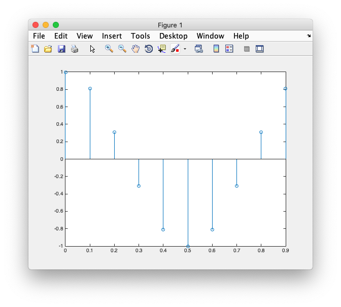
It should look like the following:
That is, it modulates one cycle of a sinusoid in one second of time. Let's get right down to business and see what the Fourier transform of the signal looks like. We do this by taking the Fast Fourier Transform (which is, well, a fast way of computing the Fourier transform of a discrete signal.
clf;
stem(0:length(sig)-1,abs(fft(sig)));
xlabel('Frequency component (cycles)');
ylabel('Amplitude');
Note that in the plot, I set the x-axis to begin at 0. You will see why in a moment. Also, I took the absolute value of the fft, you will also see why in just a bit.
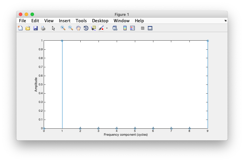
Should look like the following:
How do we interpret this graph? There is one peak at one cycle. Well, that's because the signal has one cycle in it. The magnitude of that peak actually depends on the sampling deltaT that we choose, which is not particularly important for our purposes, so let's replot adjusting for that.
clf;
stem(0:length(sig)-1,2*deltaT*abs(fft(sig)));
xlabel('Frequency component (cycles/sec)');
ylabel('Amplitude');
Now you should see the normalized peak:
Now, what is the second peak at what looks like 9 cycles/sec? Ignore it for now, it comes out from the slightly strange way in which the Fourier transform is computed which we'll get to in the Fourier transform computation tutorial.
So, why did I shift the x-axis to start at 0? That's because the first component of the Fourier transform contains the mean of the signal. This is also sometimes called the DC-offset (since electrical engineers use the Fourier transform a lot to characterize time-varying electrical signals and DC - direct current is the mean, non-time-varying part of the signal.
To understand the DC-offset part of the Fourier transform let's add a mean level to our signal and see what the Fourier transform looks like.
sig = cos(2*pi*t) + 2;
clf;
stem(0:length(sig)-1,2*deltaT*abs(fft(sig)));
xlabel('Frequency component (cycles/sec)');
ylabel('Amplitude');
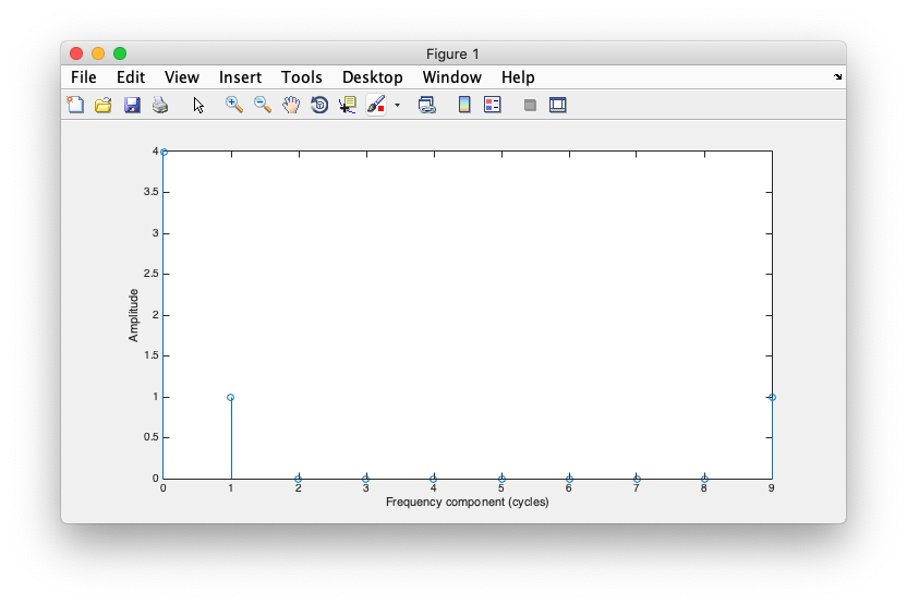
It should look like this:
Now you should see a large DC component, representing twice the offset. Why twice? Uh, again for the same reason above about having a frequency component at 9, we'll get to that in the Fourier transform computation tutorial.
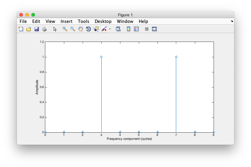
Ok, now a challenge for you. Modify the code above to have a signal that has three times the frequency of the signal we computed. What should it's Fourier transform look like? Write the code and test it out.
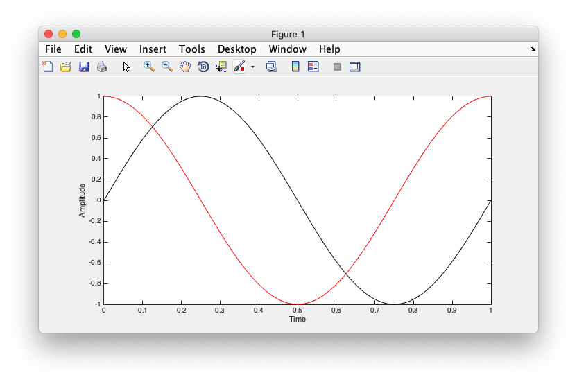
Cool. Now we know that we can use the Fourier transform to find the frequency of the sinusoid in a signal. But, what about the phase? Recall that sine and cosine are the same shape, but have a different starting point. We call that a different phase. In fact, the cosine function is just a sine function shifted by pi/2 (that's radians for 90 degrees). You can see this as follows:
clf;
% make a finer deltaT to make the curves smoother
deltaT = 0.01;
t = 0:deltaT:1-deltaT;
% plot cosine
plot(t,cos(2*pi*t),'r-');
hold on
% plot sine
plot(t,sin(2*pi*t),'k-');
xlabel('Time');
ylabel('Amplitude');
You should see the cosine function plotted in red and the sine function plotted in black.
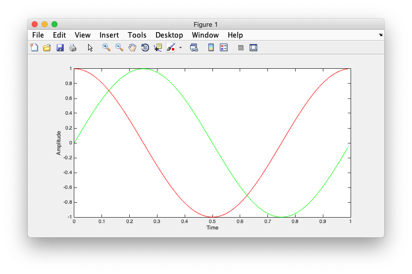
Note that they are shifted copies of each other. To confirm that they are shifted by pi/2 (or 90 degrees), plot the cos function in a different color shifted by -pi/2:
plot(t,cos(2*pi*t - pi/2),'g-');
And you will see that it completely overlaps with the cosine function.
Ok, pretty straight-forward right? Well, how does the Fourier transform represent the difference between a cosine and sine? How does it store the phase? First let's plot the Fourier transform amplitude as before for a sine function and see if it looks any different from a cosine function.
% create the sine signal
deltaT = 0.1;
t = 0:deltaT:1-deltaT;
sig = sin(2*pi*t);

% and plot
clf;
stem(0:length(sig)-1,2*deltaT*abs(fft(sig)));
xlabel('Frequency component (cycles/sec)');
ylabel('Amplitude');
Should look like exactly the same as when we did this for cosine.
So, where is the phase in the Fourier transform? You can extract it with the “angle” function (you will see why in just a bit).
% get the Fourier transform of the signal
sigFFT = 2*deltaT*fft(sig);

% set the frequency component to display
freqNum = 1;

% display the amplitude and phase at that frequency component
disp(sprintf('The amplitude for frequency %i is %f and the phase is %f (angle: %0.0f)',freqNum,abs(sigFFT(freqNum+1)),angle(sigFFT(freqNum+1)),180*angle(sigFFT(freqNum+1))/pi));
Which should give you:
The amplitude for frequency 1 is 1.000000 and the phase is -1.570796 (angle: -90)
Fourier transform of more complex signals
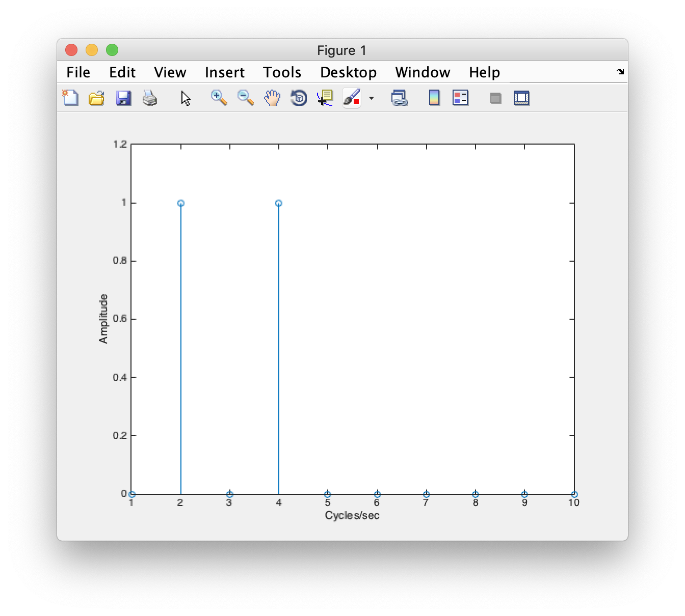
The next most complicated signal we could represent with the Fourier transform is a sum of two sinusoids. Let's take one sinusoid of frequency 2 cycles/sec and another at 4 cycles/sec. What does the sum of these look like:
% Time base (sample more to get a cleaner representation)
deltaT = 0.01;
t = 0:deltaT:1-deltaT;

% sinusoid at 2 cycles/sec
sin2 = sin(2*2*pi*t);

% sinusoid at 4 cycles/sec
sin4 = sin(4*2*pi*t);

% create signal
signal = sin2 + sin4;

% plot the signal
clf;
plot(t,signal,'k-');
xlabel('Time');
ylabel('Amplitude');

% plot the component frequencies
hold on
plot(t,sin2,'r:');
plot(t,sin4,'b:');
legend('signal','2f','4f');
What do you think the Fourier transform looks like? Just plot the first few frequencies:
Play around with different frequencies and different phases. Is it possible to make any possible signal with some sum of sinusoids of different phases and frequencies (answer is yes as you will see below!).
Now, let's go in the other direction, let's take a signal and use the Fourier transform to see how it can be composed of different sinusoids. Let's start with a square wave:
% Time base (sample more to get a cleaner representation)
deltaT = 0.01;
t = 0:deltaT:1-deltaT;

% make a square wave, starting with something that is all zero
signal = zeros(1,length(t));

% now make the central 0.5 seconds one.
signal(t > 0.25 & t < 0.75) = 1;

% plot the signal
clf;
plot(t,signal,'k-');
xlabel('Time');
ylabel('Amplitude');
% set the limits on the y-axis to more clearly see it.
set(gca,'yLim',[-0.5 1.5]);
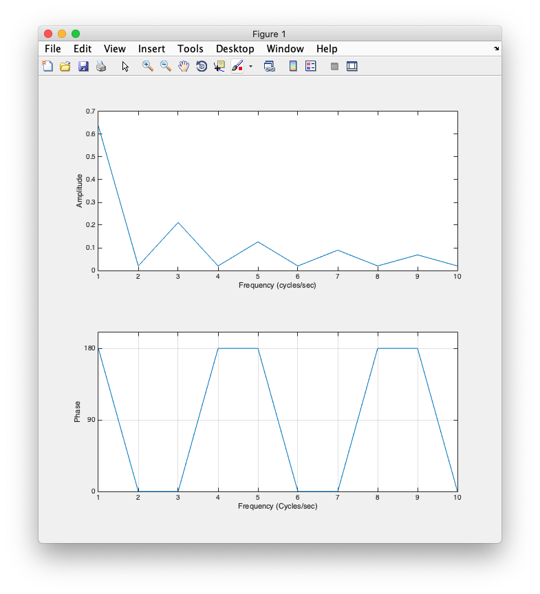
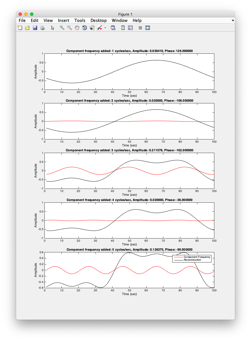
What do you think the Fourier transform will look like? First, how would you approximate the Fourier transform with one frequency and what would it's phase be? How would you get closer by adding a second frequency? A third frequency?
Does that make any sense? Try building up the signal one sinusoid at a time from the amplitude and phase you find in the Fourier transform and see what you get?
Does that make sense? Question for you. The reconstruction looks like is going from -0.5 to 0.5, yet our original signal went from 0 to 1. Why is that? What component are we missing?
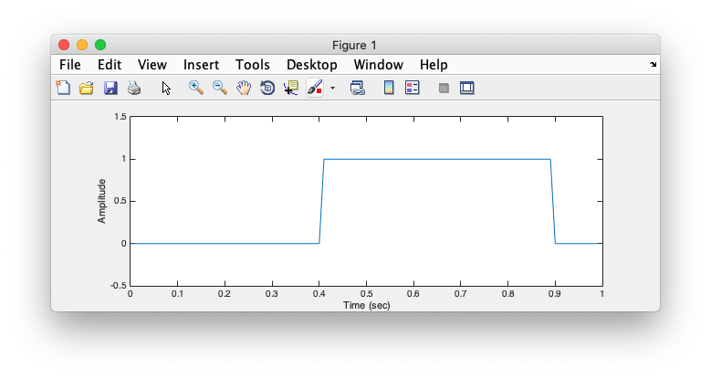
Another question for you. What would happen if you had a signal that is shifted in time, like this:
signal = zeros(1,length(t));
signal(t > 0.4 & t < 0.9) = 1;
What should change about it's Fourier transform? Amplitude? Phase?
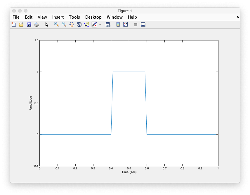
What do you think will happen if you make the peak narrower?
signal = zeros(1,length(t));
signal(t > 0.4 & t < 0.6) = 1;
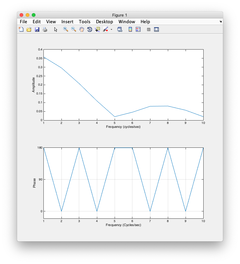
Plot it's Fourier transform as before, and look at how it reconstructs the signal.
Two dimensional Fourier transform
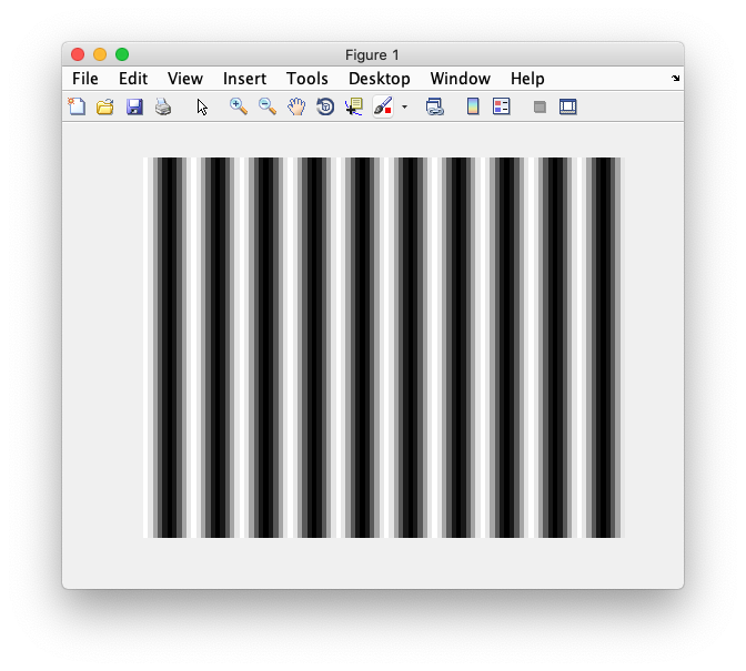
If you got all that, then making sense of two-dimensional Fourier transforms should be pretty simple. First, let's make a sinusoid in two dimensions:
% make a grid of x and y points
deltaT = 0.01;
x = [0:deltaT:1-deltaT];
y = [0:deltaT:1-deltaT];
[x y] = meshgrid(x,y);

% now set an angle and spatial frequency for the grating
theta = 0;
sf = 10;

% and compute it
grating = cos(sf*2*pi*cos(theta)*x + sf*2*pi*sin(theta)*y);

% display it
imagesc(grating);
colormap(gray);
axis off;
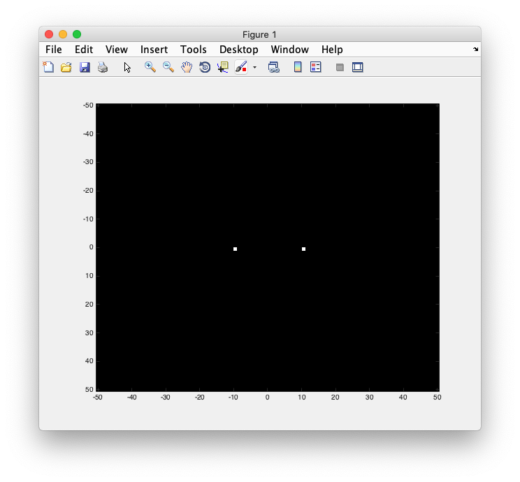
What do you think it's Fourier transform should look like? The Fourier transform is going to have two dimensions to it now. Let's take a look:
fGrating = fft2(grating);
freqRange = 1/(2*deltaT);
imagesc([-freqRange:freqRange],[-freqRange,freqRange],fftshift(abs(fGrating)));
xlabel('Spatial Frequency X (cycles/image)');
ylabel('Spatial Frequency Y (cycles/image)');
Looks like two peaks at 10 cycles/image and -10 cycles/image. Ignore (for the same reason as above), the -frequency component - it comes out because of how we compute the Fourier transform, just know that you will always have a symmetric Fourier transform.
Ok. So, now let's try to understand how this behaves. What happens if you change the spatial frequency of the image? What happens if you change the orientation? What is the coordinate system (think, radial coordinates - what does the angle, what is the radius in the Fourier transform tell you)?
Fourier transform of natural images
What does the Fourier transform of something more complex, like a natural image look like? Load the following two images (Click to bring them into their own page and then right click them and save them to somewhere you can access from Matlab):
pic01 = imread('pic01.png');
pic02 = imread('pic02.png');
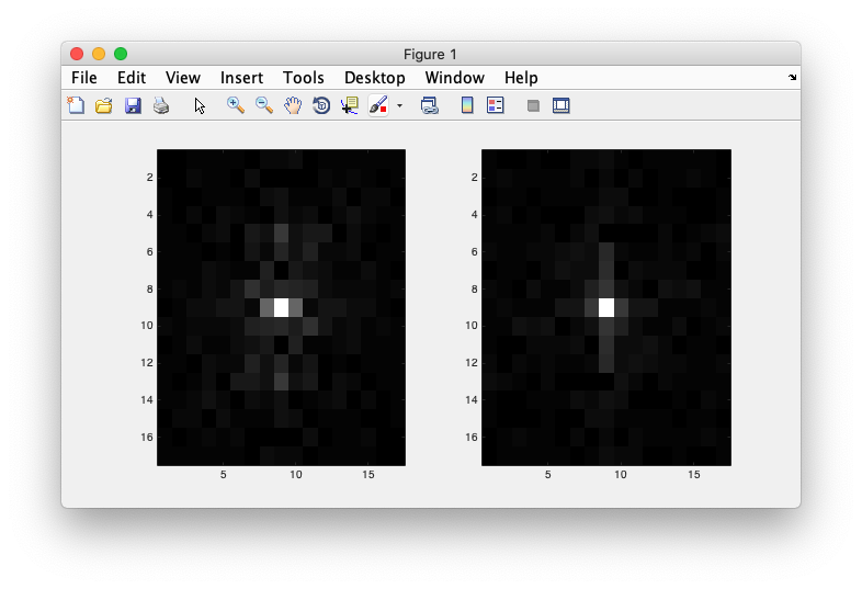
Now take their Fourier transform and display it. To see what is going on better, you may wish to remove the mean from the image (to avoid showing a large DC component) and then only show the central part of the Fourier transform with the low frequencies:
% remove the mean, so that we can the spectrum better
fPic01 = fft2(pic01-mean(pic01(:)));
fPic02 = fft2(pic02-mean(pic02(:)));

% get the center part of the Fourier transform
centerWidth = 16;
fPic01Center = fftshift(fPic01);
fPic01Center = fPic01Center((-centerWidth/2 : centerWidth/2) +1+size(fPic01Center,1)/2,(-centerWidth/2 : centerWidth/2)+1+size(fPic01Center,2)/2);

fPic02Center = fftshift(fPic02);
fPic02Center = fPic02Center((-centerWidth/2 : centerWidth/2) +1+size(fPic02Center,1)/2,(-centerWidth/2 : centerWidth/2)+1+size(fPic02Center,2)/2);

% and display
clf;
subplot(1,2,1);colormap(gray);
imagesc(abs(fPic01Center));

% display them
subplot(1,2,2);
imagesc(abs(fPic02Center));
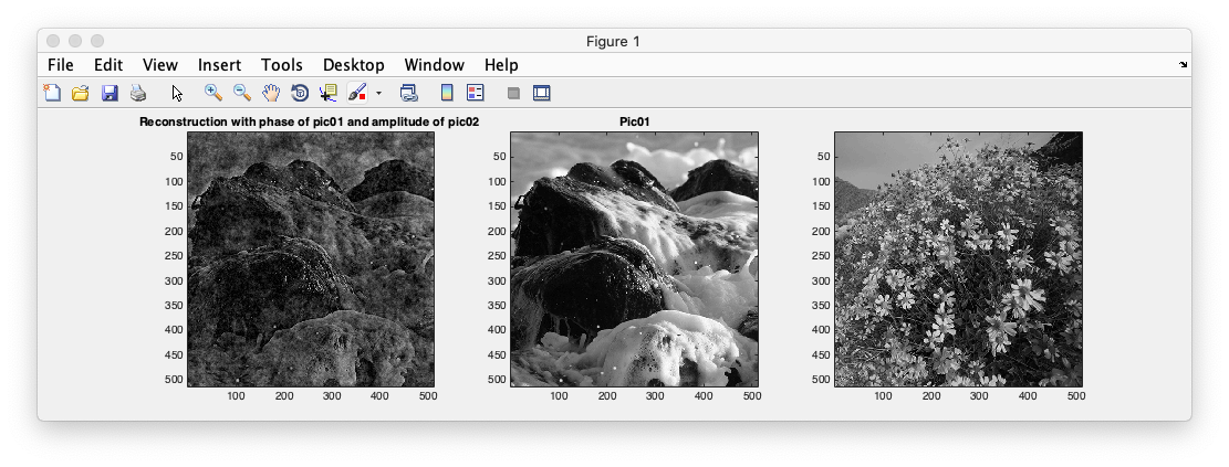
You may think that they look kinda the same. They have a central point and then everything decays pretty quickly as you move away from that point. It's like there is more power in lower spatial frequencies and less power in higher spatial frequencies. That turns out to be right in general and is a hallmark of natural images - sometimes called a 1/f drop-off. To see it even more dramatically, take the amplitude spectrum of one image and the phase spectrum of the other image and combine those. Which is more important the amplitude or the phase? Which image will it look like?
This is a little tricky - to reconstruct the image you will need to make a complex number with the amplitude from one image and the phase of the other image (we haven't yet talked about why the Fourier transform has complex numbers - just wait!)
% get amplitude and phase
fPhase = angle(fft2(pic01));
fAmplitude = abs(fft2(pic02));

% now construct a new complex number with the amplitude and phase
fReconstruct = fAmplitude .* (cos(fPhase) + sqrt(-1) * sin(fPhase));

% take inverse transform to reconstruct the image
reconstruct = abs(ifft2(fReconstruct));

% display
clf;
subplot(1,3,1);
imagesc(reconstruct);
title('Reconstruction with phase of pic01 and amplitude of pic02 ');

subplot(1,3,2);
imagesc(pic01);
title('Pic01');

subplot(1,3,3);
imagesc(pic02);
title('Pic02');
