Introduction
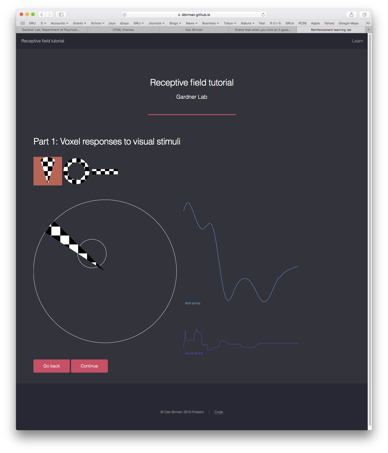
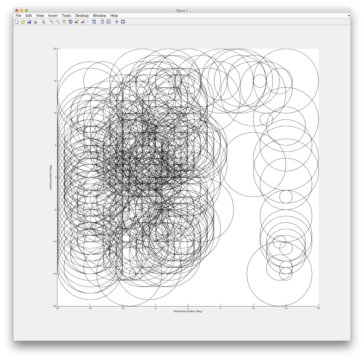
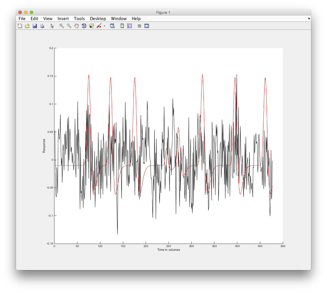
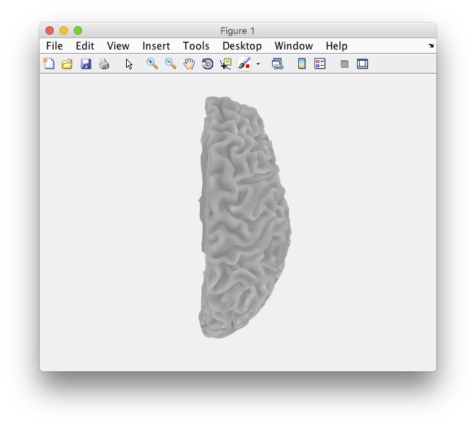
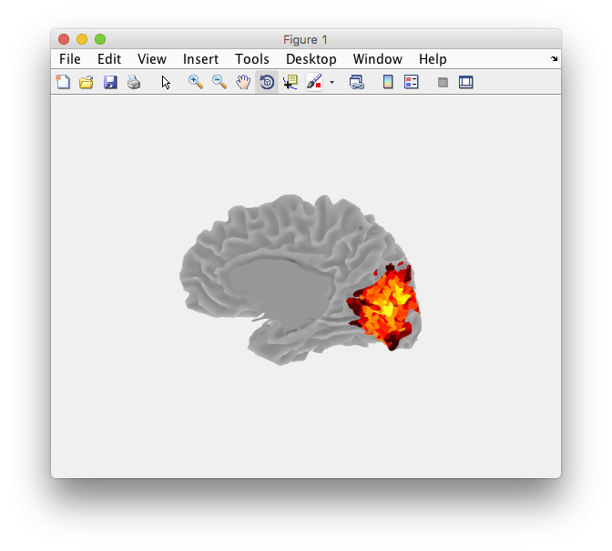
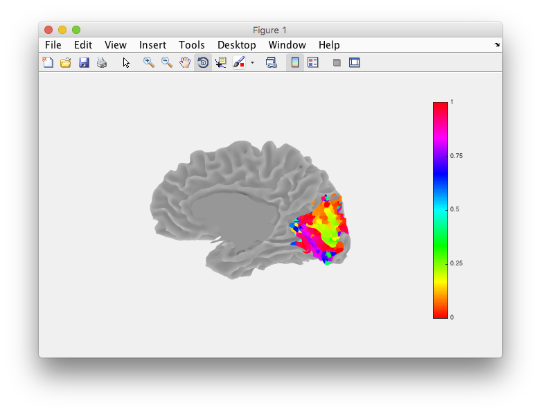
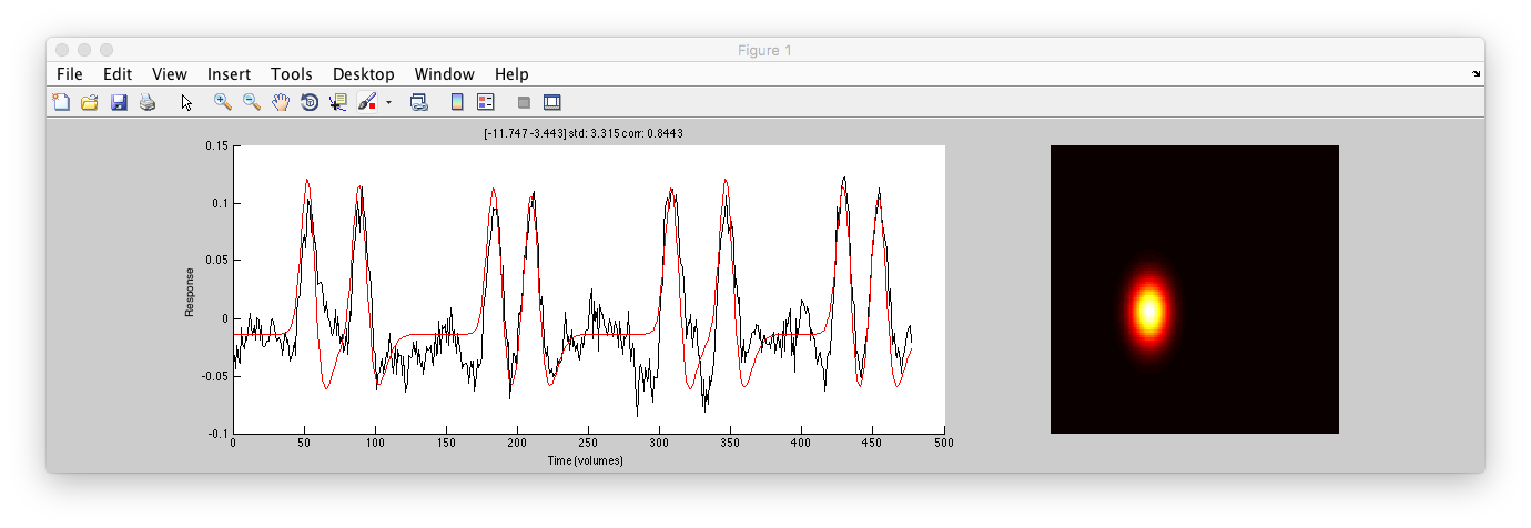
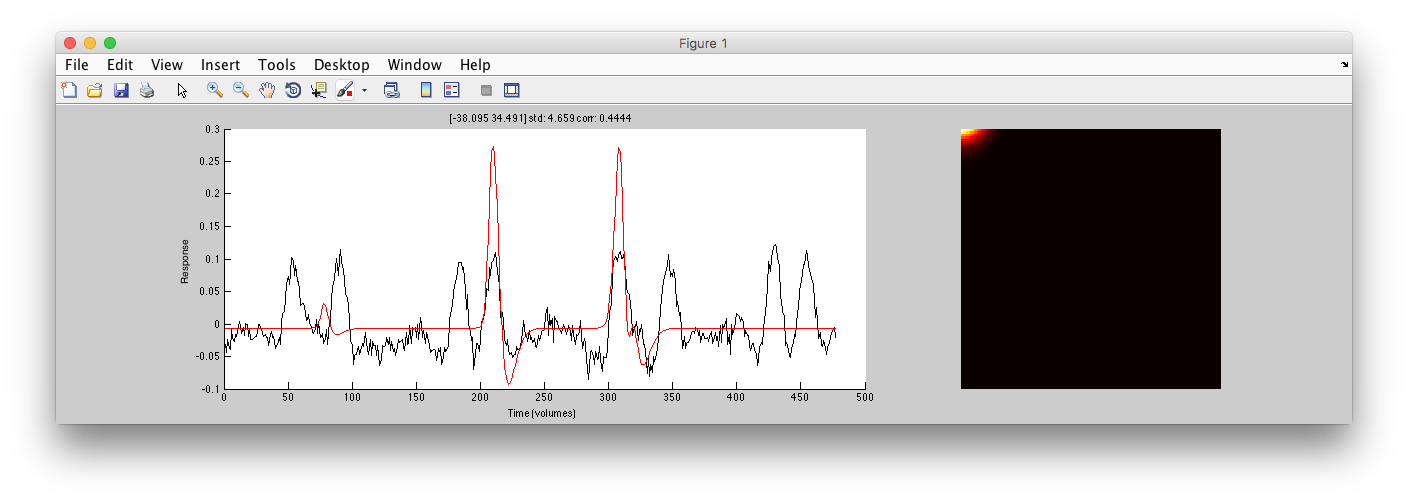
This tutorial will take you through fitting a pRF encoding model (see Dumoulin and Wandell (2008) for details) to actual data. You will write all the code to do this - either in Matlab or Python (there are worked examples of code for both Matlab and Python). You can check here for some information on how pRF fitting works and introduction to a GUI implementation. Here there will be no GUI, you will code the analysis from first principles using nothing but simple matrix computations. The full tutorial takes you through fitting a pRF model to data using a grid search, plotting the data on a triangulated cortical surface, fitting with a non-linear search algorithm (nelder-mead) and then using your fit model to decode a stimulus that was never used in training. A few snapshots from the process to give you an idea of what you will get by going through the tutorial below:
Conceptual introduction
Setup
This tutorial works in either Matlab or Python (but note that 1 section near the end on displaying results on surface is not yet implemented in Python - so will require more work on your part to write the python implementation!).
To setup for matlab, you just need to do the following:
Setup your matlab environment For those working at Stanford you can use the
corn server
Get datafiles Get the git repo with the datafiles (you will have already done this if you were following the corn instructions above)
git clone https://github.com/justingardner/pRFtutorial.git pRFtutorial
cd pRFtutorial
Start matlab
-
To setup for Python:
Get datafiles Get the git repo with the datafiles
git clone https://github.com/justingardner/pRFtutorial.git pRFtutorial
cd pRFtutorial
Start iPython
Load data# import numpy for matrix operations
import numpy
# import scipy for optimization routines
import scipy
# import scipy for the matlab reading code
import scipy.io as sio
# setup matplotlib
import matplotlib.pyplot as plt
# Load the data
pRFLoad = sio.loadmat('pRF.mat')
# get the stored matrices
stimImage = pRFLoad['stimImage']
stimX = pRFLoad['stimX']
stimY = pRFLoad['stimY']
canonical = numpy.transpose(pRFLoad['canonical'])
canonical = canonical[:,0]
c = pRFLoad['c']
v = pRFLoad['v']
t = pRFLoad['t']
tSeries = pRFLoad['tSeries'];
tSeries1 = pRFLoad['tSeries1'];
tSeries2 = pRFLoad['tSeries2'];
tSeries1 = tSeries1[:,0];
tSeries2 = tSeries2[:,0];
unknownTSeries = pRFLoad['unknownTSeries']
possibleStimImages = pRFLoad['possibleStimImages'];
base2scan = pRFLoad['base2scan']
roiScanCoords = pRFLoad['roiScanCoords'];
Look at the stimulus
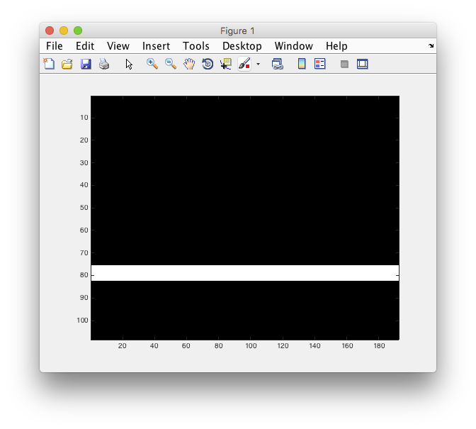
Let's start by just taking a look at the stimulus that was presented to the subject. Remember the subject was looking at the center of the screen where there was a fixation cross on which they had to perform a task (just to keep their attentional state and fixation under control) and bars moving in different directions were shown. Each frame of the image is stored as a 2D matrix that has the pixel values for each position on the screen. For this purpose, the matrix just contains 0's and 1's. Each of these 2D frames are stacked into a 3D matrix where the third dimension is time. So, good. Let's see if we can figure out what the stimulus looked like on some arbitrary frame of the stimulus, say frame 36. You should be able to do that just by looking at the values. The variable that holds the stimulus images is called: stimImage
Matlab coding hint
In matlab if you want to look at the values of a matrix just type its name. If you want to look at see all the values at one index value then you can specify that like this stimImage(:,:,36).
Probably there were too many values to look at all at once, so let's look at a subset of values between 70 and 85 and see if you can tell what the stimulus was.
Matlab coding hint
Ranges are specified as start:end, so to look at the range of values between 70 and 85, you would stimImage(70:85,70:85,36)
Python cheat sheet
stimImage[69:84,69:84,35]
Got the answer?
Answer
Ok, it might be easier to look at this as an image, so let's go ahead and display the whole thing and see what you get.
Matlab coding hint
Matlab Cheat sheet
% Display the 36th image
imagesc(stimImage(:,:,36));
% set the colormap to grayscale so that you get a black and white image
colormap(gray);
Python cheat sheet
# Display the 36th image, with the gray colormap
plt.imshow(stimImage[:,:,36],cmap="gray");
Answer
You should get something like this
Now that you can display the image, you might want to go ahead and look at the whole sequence. You can write a for loop and display each image at a time and see what it looks like.
Matlab coding hint
Do help for if you don't know how to specify a for loop. Check the size of the stim array to see how many frames there are, by using the size command and loop from 1 to that number. To make sure that the image is drawn each round of the for loop, use the command drawnow
Matlab Cheat sheet
% loop over all frames of the image
for iFrame = 1:size(stimImage,3)
  % draw it
  imagesc(stimImage(:,:,iFrame));
  % and flush graphics events
  drawnow
end
Python Cheat sheet
# This for some reason is excruciatingly slow on my machine
# so only go 30 images instead of showing the whole thing...
# get figure
fig = plt.figure()
# loop over all frames of the image
for iFrame in range(0,30):
  # draw it
  plt.imshow(stimImage[:,:,iFrame],cmap="gray");
  # flush
  fig.canvas.draw()
Good, you should have seen a bar move in various directions across the screen. That was what was shown to the subject. Run again, and count how many times a bar crossed the screen - we'll need that number as a consistency check in a following section!
Answer
Compute a gaussian receptive field
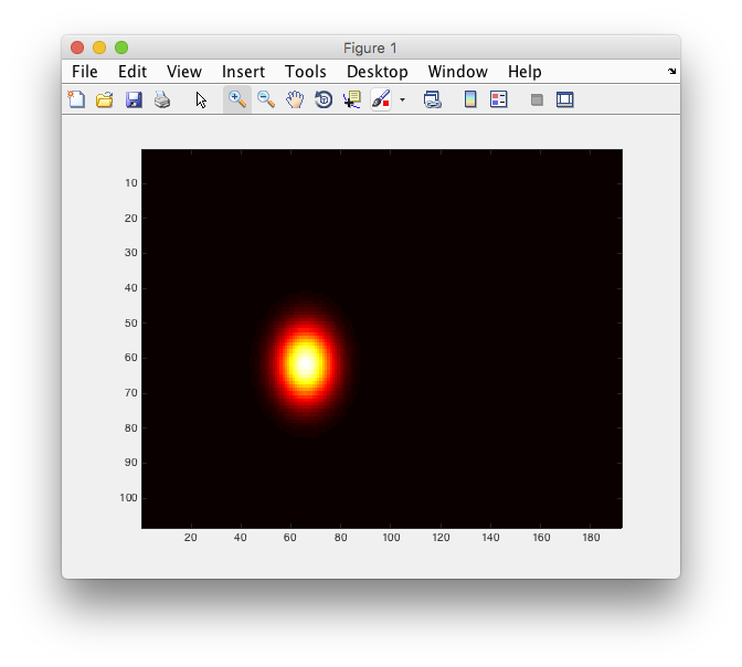
Now we need to make our encoding model. In this case it is a simple gaussian receptive field. Let's start by making an arbitrary one at the location (-12, -3) degrees (i.e. 12 degrees to the left and 3 degrees below center) We also need to set the size of the receptive field, let's do one that has a standard deviation of 3 degrees. So, first, your going need to know the equation of a gaussian, right?
Equation
gaussian(x,y) = e^{-((x-x_{center})^2 + (y-y_{center})^2)/{2\sigma^2}}
The x and y coordinates of every point of the stimulus image is in stimX and stimY, so using the 2D equation with those input points, you should be able to compute the gaussian receptive field.
Matlab coding hint
The exponential function is exp and the power function is .^ Note that the . before the ^ is used for the matrix operation
Matlab cheat sheet
% set variables for the center and width
xCenter = -12;yCenter = -3;rfstd = 3;
% compute the receptive field
rf = exp(-((stimX-xCenter).^2 + (stimY-yCenter).^2)/(2*rfstd^2));
% and display
imagesc(rf);
% use the "hot" colormap to make it prettier
colormap hot
Python cheat sheet
# set variables for the center and width
xCenter = -12
yCenter = -3
rfstd = 3
# compute the receptive field
rf = numpy.exp(-(numpy.power(stimX-xCenter,2) + numpy.power(stimY-yCenter,2))/(2*rfstd**2));
# and display
plt.imshow(rf,cmap="hot");
Answer
You should get something like this
Compute the model neural response
Now that we have the receptive field and the stimulus, it's time to compute the expected “neural response”. The amount of overlap between the stimulus and the receptive will govern the neural response. (For our purposes we won't consider any of the dynamics of neural responses themselves - e.g. transients, adaptation, offset responses, etc etc) To compute the overlap, we just take a point by point multiplication of the stimulus image with the receptive fields and sum across all points. You should now try to compute that for every time point in the stimulus image.
Matlab coding hint
To compute the point-by-point multiplication between two matrices you use the operator .* to sum across all points in the matrix you use the function sum. Note that to sum over all points, you need to use the sum operator twice (since each time it will sum over one dimension). Try to first compute the response for one frame, and then once you have that working, then do a for loop
Matlab cheat sheet
% loop over frames
for iFrame = 1:size(stimImage,3)
  % compute overlap
  rfStimulusOverlap = stimImage(:,:,iFrame) .* rf;
  % sum over all points
  modelNeuralResponse(iFrame) = sum(sum(rfStimulusOverlap));
end
% plot what we got
plot(modelNeuralResponse);
Python cheat sheet
# init array
modelNeuralResponse = numpy.zeros(stimImage.shape[2])
# loop over frames
for iFrame in range(0,stimImage.shape[2]):
  # compute overlap
  rfStimulusOverlap = numpy.multiply(stimImage[:,:,iFrame],rf);
  # sum over all points
  modelNeuralResponse[iFrame] = numpy.sum(rfStimulusOverlap);

# plot what we got
plt.clf()
plt.plot(modelNeuralResponse);
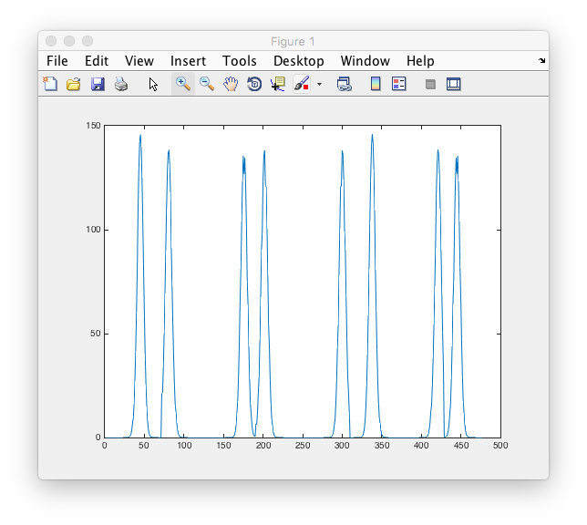
How many peaks in this simulated neural response do you see? Does it match the number of times there was a bar moving across the visual field that you counted above?
Answer
You should see something like this
Compute the model BOLD response
Now we have to convert this model neural response into a model BOLD response. The model that we use for this is that the BOLD response is a convolution of a canonical hemodynamic response function with the neural response. So, go ahead and compute the convolution of the model neural response with the canonical hemodynamic response function (we have provided one in the variable called canonical
Matlab coding hint
Do a help on the function conv
Matlab Cheat sheet
% do the convolution
modelBoldResponse = conv(modelNeuralResponse,canonical);
% and display
plot(modelBoldResponse);
Python Cheat sheet
# do the convolution
modelBoldResponse = numpy.convolve(modelNeuralResponse,canonical);
# and display
plt.clf()
plt.plot(modelBoldResponse);
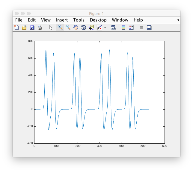
Answer
Should look like the following
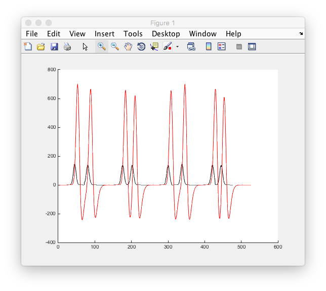
Ok. Sanity check (always good to check that things are making sense as you go along as much as possible). Plot the neural response on the same graph as the bold response and see if you they make sense. In particular, the bold response should start after the neural response and last longer, right?
Matlab coding hint
Use clf to clear the figure. To plot two things on the same graph, use hold on. The plot command can be used to plot in different colors. Do a help on plot
Matlab Cheat sheet
clf;
hold on;
plot(modelNeuralResponse,'k-');
plot(modelBoldResponse,'r-');
Python Cheat sheet
plt.clf();
plt.plot(modelNeuralResponse,'k-');
plt.plot(modelBoldResponse,'r-');
Answer
Should look like the following
Ok. Looks good? What about at the very end. Do you notice that the BOLD response lasts longer than the neural response? That's because the conv command returns a vector longer than the original response. We don't want that last piece, so remove it from the bold model response (otherwise, dimensions won't match for the calculations we do later). Also, let's take the transpose of this modelBoldResponse (also important for matching dimensions up later)
Matlab coding hint
length can be used to find the length of a vector. To get the subset of a vector, use the techniques we used above to get a portion of the stim image. To take the transpose of a vector use '
Matlab cheat sheet
modelBoldResponse = modelBoldResponse(1:length(modelNeuralResponse))';
Python cheat sheet
modelBoldResponse = numpy.transpose(modelBoldResponse[0:modelNeuralResponse.shape[0]]);
Compare the model to measured responses
Ok. So, we can compute the model BOLD response for a specific receptive field - now we want to know how to compare that to measured responses. We're going to use the time-point by time-point correlation between the model and the measured responses. Correlation is a nice measure to work with, since it isn't affected by the magnitude of responses. Remember that we haven't really done anything to make the units of the model match the units of response (look back at the units you have for the model BOLD response - typical BOLD responses are about 1 or 2% signal change - is that the size of the fluctuations you have in the model? (no. right!). We could fit a parameter there so that we get the model output to match in magnitude to the BOLD response (how would you do that?), but here we'll just ignore the whole issue by using correlation. Ok, we have two actual time series for you to work with tSeries1 and tSeries2 (they were measured from a subject viewing the stimuli). Go ahead and compute the correlation between these time series and the measured bold response from above. What do you get? For which tSeries is this model rf a good model for?
Matlab coding hint
Matlab cheat sheet
corr(tSeries1,modelBoldResponse)
corr(tSeries2,modelBoldResponse)
Pyton cheat sheet
numpy.corrcoef(tSeries1,modelBoldResponse)[0,1]
numpy.corrcoef(tSeries2,modelBoldResponse)[0,1]
Answer
The correlation for tSeries1 is: 0.839672
The correlation for tSeries2 is: 0.1711145
So, the model RF is best for tSeries1.
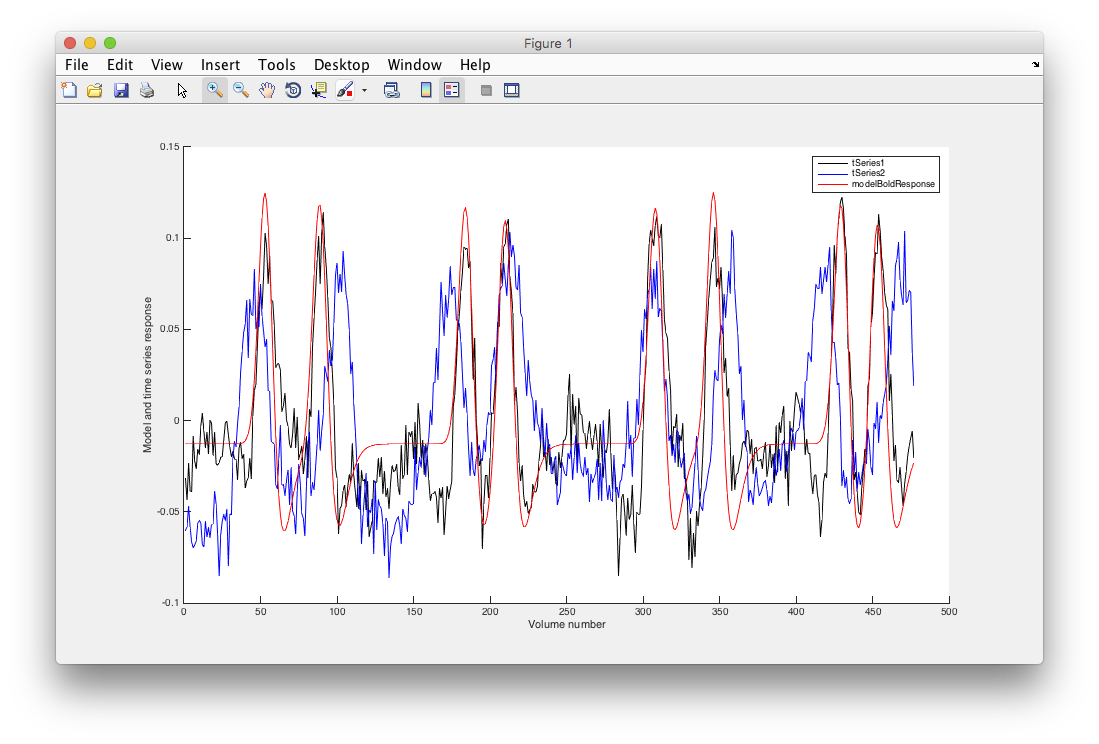
Ok. Let's confirm that visually, by plotting the model and the time series together and see that they match. Now, we have to worry a little bit about the magnitudes which are going to be different between the model and the actual bold responses - let's handle this by normalizing the model and the bold responses to have zero mean and vector length of 1 (i.e. subtract the mean and divide by the square root of the sum of squares). This normalization is useful since later it will allow us to compute the correlation efficiently. Probably worth noting here an important maxim. Anything you do to your data - you are going to need to do to the model as well. So if we divide by the mean of the bold responses, then divide by the mean in the model as well. If you high pass filter your data, then you need to high pass filter your data. Ok. Go ahead and do that and then plot the model and the time series.
Matlab coding hint
The square of every value in an array can be computed using .^2. You already know about sum and square root is sqrt
Matlab cheat sheet
% normalize time series
tSeries1 = tSeries1-mean(tSeries1);
tSeries1 = tSeries1/sqrt(sum(tSeries1.^2));
tSeries2 = tSeries2-mean(tSeries2);
tSeries2 = tSeries2/sqrt(sum(tSeries2.^2));
% everything that is done to the data should also be done to the model
modelBoldResponse = modelBoldResponse-mean(modelBoldResponse);
modelBoldResponse = modelBoldResponse/sqrt(sum(modelBoldResponse.^2));
% now plot
clf;
hold on;
plot(tSeries1,'k-');
plot(tSeries2,'b-');
plot(modelBoldResponse,'r-');
% label stuff
xlabel('Volume number');
ylabel('Model and time series response');
legend('tSeries1','tSeries2','modelBoldResponse')
Python cheat sheet
# normalize time series
tSeries1 = tSeries1-numpy.mean(tSeries1);
tSeries1 = tSeries1/numpy.sqrt(numpy.sum(numpy.power(tSeries1,2)));
tSeries2 = tSeries2-numpy.mean(tSeries2);
tSeries2 = tSeries2/numpy.sqrt(numpy.sum(numpy.power(tSeries2,2)));
# everything that is done to the data should also be done to the model
modelBoldResponse = modelBoldResponse-numpy.mean(modelBoldResponse);
modelBoldResponse = modelBoldResponse/numpy.sqrt(numpy.sum(numpy.power(modelBoldResponse,2)));
# now plot
plt.clf()
plt.plot(tSeries1,'k-')
plt.plot(tSeries2,'b-')
plt.plot(modelBoldResponse,'r-')
# label stuff
plt.xlabel('Volume number')
plt.ylabel('Model and time series response')
plt.legend(['tSeries1','tSeries2','modelBoldResponse'])
So, should be a great match for tSeries1 and a pretty bad match for tSeries2.
Answer
Find the best model for a time series
Ok, so of course the example above for tSeries1 was totally cooked - I gave you the parameters that would pretty closely match the response. How can we find the best parameters for tSeries2 (and in general any time series for which we don't know what the receptive field parameters are). After all, that's the whole goal of what we are doing right? To figure out what the receptive field model is that best explains the responses of each voxel. We'll first do a quick and dirty way to get close to the right parameters by doing a grid search. What's a grid search? It's just forming a grid of parameters and testing to see which model parameters on this grid give a model response that best fits the voxel. In this case, our grid will be over x and y position of the receptive field and the width (standard deviation). Let's try x and y from -15 to 15 degrees in steps of 1 and standard deviations from 1 to 5 in steps of 1. We'll start by computing receptive fields for all combinations of these parameters and putting them all into a single giant matrix of model responses. Each row of this matrix will contain a model response with one parameter combination. So, if the length of a model response in n and there are k different combinations, you should create a k x n matrix. Also, remember to keep which model parameters made which model response in the k x n matrix, so store those in another k x 3 matrix (the three is for the three different parameters). Got it?
Matlab coding hint
You should be able to nest three for loops (one for x, one for y and one for standard deviation) and then put each model response you calculate as above in each row of a matrix. Different ways to do this, but easiest might be to start a variable before your for loop with the index into this matrix modelNum=1; and then put model responses into the modelResponses(modelNum,:) = computed model response like above. Then increment modelNum in the loop. Also, to speed things up it is worthwhile initializing the modelResponses matrix with enough space to hold all the model responses - otherwise matlab has to dynamically reallocate space on each loop iteration, making it slow. You can precompute space by setting modelResponses - nan(k,n) where k and n are set to appropriate sizes
Matlab cheat sheet
%%%%%%%%%%%%%%%%%%%%%%%%%%%%%%%%%
% Note that running this code may take a minute or two to complete...
%%%%%%%%%%%%%%%%%%%%%%%%%%%%%%%%%
% init space for modelResponses and params
k = 4805;n = size(stimImage,3);
modelResponses = nan(k,n);
params = nan(k,3);
% index for where to put each model response
modelNum = 1;
% loop over x
for x = -15:15
  % loop over y
  for y = -15:15
    % loop over s
    for s = 1:5
       % get the rf
       rf = exp(-((stimX-x).^2 + (stimY-y).^2)/(2*s^2));
       % instead of looping over frames, we use a slight trick
       % to do this as a matrix operation - we replicate the rf for
       % each time point and then compute the sum over all points in one pass
       % matlab is very fast with matrix operations, so if you can rewrite any
       % loop as a matrix operation it will generally speed things up significantly
       modelNeuralResponse = squeeze(sum(sum(stimImage .* repmat(rf,1,1,n))));
       % do the convolution
       modelBoldResponse = conv(modelNeuralResponse,canonical);
       % trim length
       modelBoldResponse = modelBoldResponse(1:n)';
       % normalize
       modelBoldResponse = modelBoldResponse-mean(modelBoldResponse);
       modelBoldResponse = modelBoldResponse/sqrt(sum(modelBoldResponse.^2));
       % now place into giant matrix
       modelResponses(modelNum,:) = modelBoldResponse;
       % keep the params
       params(modelNum,:) = [x y s];
       % update modelNum
       modelNum = modelNum + 1;
    end
  end
  % display something so that we know that things are progressing
  disp(sprintf('Computed receptive fields for x = %i',x));
end
Python cheat sheet
# to paste this into the buffer, copy the text below and then in the
# ipython window type %paste and hit enter

#################################
# Note that running this code may take a minute or two to complete...
#################################
# init space for modelResponses and params
k = 4805
n = stimImage.shape[2]
modelResponses = numpy.zeros([k,n])
params = numpy.zeros([k,3])
# index for where to put each model response
modelNum = 1
# loop over x
for x in range(-15,15):
  # loop over y
  for y in range(-15,15):
    # loop over s
    for s in range(1,5):
       # compute the receptive field
       rf = numpy.exp(-(numpy.power(stimX-x,2) + numpy.power(stimY-y,2))/(2*s**2))
       # init array
       modelNeuralResponse = numpy.zeros(stimImage.shape[2])
       # loop over frames
       for iFrame in range(0,stimImage.shape[2]):
         # compute overlap
         rfStimulusOverlap = numpy.multiply(stimImage[:,:,iFrame],rf)
         # sum over all points
         modelNeuralResponse[iFrame] = numpy.sum(rfStimulusOverlap)
       # do the convolution
       modelBoldResponse = numpy.convolve(modelNeuralResponse,canonical)
       # trim length
       modelBoldResponse = numpy.transpose(modelBoldResponse[0:modelNeuralResponse.shape[0]])
       # normalize
       modelBoldResponse = modelBoldResponse-numpy.mean(modelBoldResponse)
       modelBoldResponse = modelBoldResponse/numpy.sqrt(numpy.sum(numpy.power(modelBoldResponse,2)))
       # now place into giant matrix
       modelResponses[modelNum,:] = modelBoldResponse
       # keep the params
       params[modelNum,:] = [x,y,s]
       # update modelNum
       modelNum = modelNum + 1
  # display something so that we know that things are progressing
  print('Computed receptive fields for x =',x)
Ok, now that we have these matrix of modelResponses for a grid of different parameter settings, let's do some sanity checks to make sure we have what we think we have (As you see, I'm a big believe in sanity checks!). First, plot a few model responses. Do they have 8 peaks as you expect? Second, remember that tSeries1 was best correlated with the rf we calculated above for [-12, -3] and a standard deviation of 3? That should be true here to. First, go find which modelNum has those parameters.
hint
Now compute the correlation between tSeries1 and tSeries2 for that modelRow number, you should be able to replicate the correlation numbers from above. Note that you will need to take the transpose of the modelResponses to make the dimensions work out correctly.
Matlab cheat sheet
% check correlation with tSeries1
corr(modelResponses(528,:)',tSeries1)
% check correlation with tSeries2
corr(modelResponses(528,:)',tSeries2)
Python cheat sheet
# check correlation with tSeries1
numpy.corrcoef(modelResponses[411,:],tSeries1)[0,1]
# check correlation with tSeries2
numpy.corrcoef(modelResponses[411,:],tSeries2)[0,1]
Everything check out? Good. Now let's find a better set of parameters for tSeries2. We can do this by computing the correlation of tSeries2 against every model in the matrix. We could build a for loop to do this, but it's actually much simper then that. Correlation is computed as the dot product of two unit length vectors (remember I told you that normalization was going to be useful?) So, all we have to do is compute the matrix product of the modelResponses matrix with the tSeries and we will get all the correlation values we need. So, let's try first with tSeries1 and confirm we get back the model that we already know is best. Find the correlation that is maximum - this should be the one with parameters [-12, -3] and standard deviation of 3.
Matlab cheat sheet
% compute correlation with every modelResponses by taking the matrix product
r = modelResponses*tSeries1;
% now find the correlation that is highest
[maxR bestModel] = max(r);
% check what those parameters are
params(bestModel,:)
Python cheat sheet
# compute correlation with every modelResponses by taking the matrix product
r = numpy.matmul(modelResponses,tSeries1);
# now find the correlation that is highest
maxR = numpy.max(r)
bestModel = numpy.argmax(r)
# check what those parameters are
params[bestModel,:]
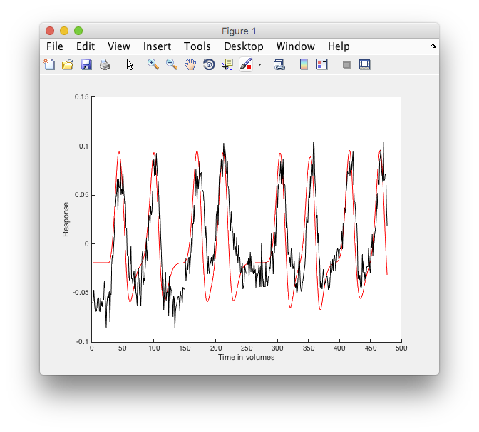
If that worked, then try it with the other time series, tSeries2, and you should get a model with good fit. Go ahead and plot that best model against tSeries2 to confirm that is the case.
Matlab cheat sheet
% compute correlation with every modelResponses by taking the matrix product
r = modelResponses*tSeries2;
% now find the correlation that is highest
[maxR bestModel] = max(r);
% check what those parameters are
params(bestModel,:)
% plot the model and the response
clf;hold on;
plot(modelResponses(bestModel,:),'r-');
plot(tSeries2,'k-');
% some labels
xlabel('Time in volumes');
ylabel('Response');
legend('Best model','tSeries2');
Python cheat sheet
# compute correlation with every modelResponses by taking the matrix product
r = numpy.matmul(modelResponses,tSeries2);
# now find the correlation that is highest
maxR = numpy.max(r)
bestModel = numpy.argmax(r)
# check what those parameters are
params[bestModel,:]
# plot the model and the response
plt.clf()
plt.plot(modelResponses[bestModel,:],'r-');
plt.plot(tSeries2,'k-');
# some labels
plt.xlabel('Time in volumes');
plt.ylabel('Response');
plt.legend(['Best model','tSeries2']);
Answer
The best fitting parameters are [-3, -9] with a standard deviation of 5
Fit a bunch of voxels
Ok, so that's a pretty rough and ready way to fit (using a grid search - we'll get more precise values in a later section), but it's good enough that we can go ahead and fit a whole bunch of voxels and plot them to see if we can see maps of visual cortex. To start with let's get the best model fit for all the tSeries that we have. It's real simple, just do the matrix multiplication against the modelResponses matrix to get the correlation, and then use max to figure out which modelResponse each tSeries gives the best fit. The hardest part is simply getting the matrix dimensions correct. modelResponse is a m x n matrix (with m models and n volumes), and tSeries is v x n (v voxels by n volumes), so to take the matrix multiplication you need to take the transpose of tSeries. This will create a k x v matrix where k is the number of models and v is the number of voxels. You want to take the max of this matrix along the model responses dimension - i.e. the largest correlation for each voxel, which is the first dimension. If you accept two arguments from the max operator it will give you both the maximum correlation (a number that is useful for evaluating model fit) and the index of which model produced that maximum value. Try it out.
Matlab coding hint
Use ' to take transpose of the tSeries
Matlab cheat sheet
% do the grid search to find the model with the best
% correlation with each time series
[maxR bestModel] = max(modelResponses*tSeries');
Python cheat sheet
# do the grid search to find the model with the best
# correlation with each time series
r = numpy.matmul(modelResponses,numpy.transpose(tSeries))
maxR = numpy.max(r,0)
bestModel = numpy.argmax(r,0)
Ok. You guessed it - now we need to do a sanity check to make sure that we got the right thing. We know that the best model for tSeries1 was 528, so let's make sure that's true for this computation to. In the tSeries matrix, the tSeries1 is the 134 response. So check maxR and bestModel and make sure that you get the expected values.
And another sanity check. Receptive fields in primary visual cortex should all be contralateral. The set of voxels you just fit were all in the right visual cortex - so let's make sure that the receptive fields found were all in the left visual field. To do that, let's figure out how to plot the contour of a receptive field. Remember the equation we used for the gaussian? Let's plot a set of x,y points for the one standard deviation contour. How do we do that? We can do that by finding all the y vales for a set of x values using the equation. So, take all x values from -std to +std and find the appropriate y-values. You will need to rearrange the gaussian equation to get y as a function of x.
hint
Find out what the equation equals when x is one std and y is 0. Set the gaussian equation equal to that and take the logarithm of both sides to get rid of the exponent
Got it? Then start by plotting a gaussian contour with center at, say, [-5, +3] and std = 3.
Matlab cheat sheet
% set the center and std
centerX = -5;centerY = 3; rfstd = 3;
% set the x-values
x = -rfstd:0.1:rfstd;
% clear the graph
clf;hold on
% plot the positive y-values
plot(x+centerX,sqrt(rfstd^2 - x.^2)+centerY,'k-');
% plot the negative y-values
plot(x+centerX,-sqrt(rfstd^2 - x.^2)+centerY,'k-');
Python cheat sheet
# set the center and std
centerX = -5
centerY = 3
rfstd = 3
# set the x-values
x = numpy.linspace(-rfstd,rfstd,100)
# clear the graph
plt.clf()
# plot the positive y-values
plt.plot(x+centerX,numpy.sqrt(numpy.power(rfstd,2) - numpy.power(x,2))+centerY,'k-');
# plot the negative y-values
plt.plot(x+centerX,-numpy.sqrt(numpy.power(rfstd,2) - numpy.power(x,2))+centerY,'k-');
You should see something that looks like a circle. If you got that, then now go ahead and use that code to plot all the contours for all the fit receptive fields.
Matlab cheat sheet
% clear the figure
clf; hold on;
% cycle over voxels
for iVox = 1:length(bestModel)
  % get the parameters
  centerX = params(bestModel(iVox),1);
  centerY = params(bestModel(iVox),2);
  rfstd = params(bestModel(iVox),3);
  % now plot the RF
  % set the x-values
  x = -rfstd:0.1:rfstd;
  % plot the positive y-values
  plot(x+centerX,sqrt(rfstd^2 - x.^2)+centerY,'k-');
  % plot the negative y-values
  plot(x+centerX,-sqrt(rfstd^2 - x.^2)+centerY,'k-');
end
% set axis and label
axis([-20 20 -20 20]);
xlabel('Horizontal position (deg)');
ylabel('vertical position (deg)');
Python cheat sheet
# You may want to use the %paste trick here...

# clear the figure
plt.clf()
# cycle over voxels
for iVox in range(0,bestModel.size):
  # get the parameters
  centerX = params[bestModel[iVox],0];
  centerY = params[bestModel[iVox],1];
  rfstd = params[bestModel[iVox],2];
  # now plot the RF
  # set the x-values
  x = numpy.linspace(-rfstd,rfstd,100)
  # plot the positive y-values
  plt.plot(x+centerX,numpy.sqrt(numpy.power(rfstd,2) - numpy.power(x,2))+centerY,'k-');
  # plot the negative y-values
  plt.plot(x+centerX,-numpy.sqrt(numpy.power(rfstd,2) - numpy.power(x,2))+centerY,'k-');

# set axis and label
plt.xlim(-20,20)
plt.ylim(-20,20)
plt.xlabel('Horizontal position (deg)');
plt.ylabel('vertical position (deg)');
Does it look like most of the receptive fields are in the left visual field, as expected?
answer
It's close, but not perfect - there are a few weird ones in the right. That could be because these are not fit well and they are just due to noise. So, check that (again, a good sanity check!). Modify your code for plotting the pRF contours so that it only plots pRFs that have a correlation of greater than, say, 0.4 (remember that we calculated the best correlation above and left it in the variable maxR). Are the receptive fields now in the correct visual field?
Matlab cheat sheet
% clear the figure
clf; hold on;
% cycle over voxels
for iVox = 1:length(bestModel)
  if maxR(iVox) > 0.4
    % get the parameters
    centerX = params(bestModel(iVox),1);
    centerY = params(bestModel(iVox),2);
    rfstd = params(bestModel(iVox),3);
    % now plot the RF
    % set the x-values
    x = -rfstd:0.1:rfstd;
    % plot the positive y-values
    plot(x+centerX,sqrt(rfstd^2 - x.^2)+centerY,'k-');
    % plot the negative y-values
    plot(x+centerX,-sqrt(rfstd^2 - x.^2)+centerY,'k-');
  end
end
% set axis and label
axis([-20 20 -20 20]);
xlabel('Horizontal position (deg)');
ylabel('vertical position (deg)');
Python cheat sheet
# You may want to use the %paste trick here...

# clear the figure
plt.clf()
# cycle over voxels
for iVox in range(0,bestModel.size):
  if maxR[iVox] > 0.4:
    # get the parameters
    centerX = params[bestModel[iVox],0];
    centerY = params[bestModel[iVox],1];
    rfstd = params[bestModel[iVox],2];
    # now plot the RF
    # set the x-values
    x = numpy.linspace(-rfstd,rfstd,100)
    # plot the positive y-values
    plt.plot(x+centerX,numpy.sqrt(numpy.power(rfstd,2) - numpy.power(x,2))+centerY,'k-');
    # plot the negative y-values
    plt.plot(x+centerX,-numpy.sqrt(numpy.power(rfstd,2) - numpy.power(x,2))+centerY,'k-');

# set axis and label
plt.xlim(-20,20)
plt.ylim(-20,20)
plt.xlabel('Horizontal position (deg)');
plt.ylabel('vertical position (deg)');
Cool. One last thing to check here, if it really is the case that those pRFs with low correlation are bad fits, then you should be able to go find one of those voxels with a low r and plot it against the model time course and see that it doesn't look good.
Matlab cheat sheet
% find all the voxels with correlations greater than 0.4
find(maxR<0.4)
% let's just choose an arbitrary one to look at, say voxel 58
checkVoxel = 58;
% find out what it's parameters were
params(bestModel(checkVoxel),:)
% plot it's time series - make sure you have which dimension is which, correct!
clf;hold on
plot(tSeries(checkVoxel,:),'k-');
plot(modelResponses(bestModel(checkVoxel),:),'r-');
% label graph
xlabel('Time in volumes');
ylabel('Response');
Python cheat sheet
# find all the voxels with correlations greater than 0.4
numpy.where(maxR<0.4)
# let's just choose an arbitrary one to look at, say voxel 57
checkVoxel = 57;
# find out what it's parameters were
params[bestModel[checkVoxel],:]
# plot it's time series - make sure you have which dimension is which, correct!
plt.clf()
plt.plot(tSeries[checkVoxel,:],'k-');
plt.plot(modelResponses[bestModel[checkVoxel],:],'r-');
% label graph
plt.xlabel('Time in volumes');
plt.ylabel('Response');
Answer
And, there's a pretty important lesson here (which is sometimes forgotten). If your fit is bad (in this case low correlation) then the parameters you fit cannot be interpreted! So, always (whether you are doing an encoding model or a GLM or whatever) - you have to check goodness of fit before trying to extrapolate anything from what parameters you got. To use technical terms, if goodness-of-fit is crap then your parameter estimates will be crap too.
Plot values on surface
Now, let's see what this analysis looks like on the cortex. Let's project these values on to a cortical surface and take a look. First, we need to know how to draw a cortical surface. Take a quick look at surfaces and flat maps and make sure you understand the idea of triangulated meshes. Ok. Are you an expert now? Let's try and display a surface. We have the surface vertices in the variable v, the triangles (or faces) in t, and the colors for each vertex in c. You should be able to use the patch command, as follows:
clf
% draw the surface
patch('vertices',v,'faces',t,'FaceVertexCData',c,'facecolor','interp','edgecolor','none')
% set the axis to make it display nicely
axis equal
axis off
If you click the circular arrow tool in the figure, you should be able to use the mouse to turn the surface around to view it from any angle you like.
Answer
Ok, but how do we plot the values from the pRF fit on to this surface. Let's first do this for the correlation values (that way we can see what part of cortex is the best fit. We are going to need to do a coordinate transform to know how to put the values from voxels take on the PRF scan into the coordinates of the surface. Take a quick look at this page on coordinate transforms to get oriented to how this works. Ok, you back? Then your should have learned that you can apply a 4×4 matrix transformation to coordinates that have a one added to them to go from one voxel coordinates to another. In this case, we will go from the coordinates of the surface (which comes from the voxels of the original 3D canonical anatomy) to coordinates of the pRF scan (note that when you want to color the vertices of the surface, you want to go in this direction and not from the scan to the base coordinates - since multiple base coordinates may correspond to a single scan coordinate - since the voxels are bigger in the scan then in the 3D canonical). Ok, so let's try that once and see how it goes. Pick any vertex (remember that the vertices of the surface are in the coordinate frame of the canonical scan) and convert it into coordinates of the scan. The transform matrix is in the variable base2scan. Remember that order matters here (the xform matrix comes first before the coordinates). And make sure you get the dimensions right (i.e. the xform is a 4×4, so that coordinate has to be a 4×1)!
Cheat sheet
% pick an arbitrary vertex
vertexIndex = 1640;
% and compute where it lives in the scan
vertexScanCoords = base2scan * [v(vertexIndex,:) 1]'
Answer
vertexScanCoords =

          39.0905160547765
          75.1531615844523
          21.9470110421143
                         1
Now that we know where it lives in the scan, we need to figure out if it is close to any of the voxels that we have computed the pRF for. To do that, compute the euclidean distance from each one of the roiScanCoords and see which one it is closest to. Note that roiScanCoords is a 3xr matrix where r is the number of voxels in the roi.
Cheat sheet
% loop over voxels in roi
for iVox = 1:size(roiScanCoords,2)
   % compute distance
   d(iVox) = sqrt(sum((vertexScanCoords(1:3) - roiScanCoords(1:3,iVox)).^2));
end
% now see which is the closest.
[minD minIndex] = min(d)
Answer
minD =

         0.185632585453267


minIndex =

    50
Ok. Good, now we know how to find which voxel is closest, we should be able to set the color of that vertex accordingly . Let's choose a value from the hot colormap according to the r value. To do this, we get the hot colormap for 256 colors - and then map the r value (0-1) into the range `1:256. Try that out.
Matlab coding hint
Do a help on hot. You may also need to use ceil.
Cheat sheet
% get the hot colormap
nColors = 256;
hotmap = hot(nColors);
% get the correlation value of the closest voxel
r = maxR(minIndex);
% convert r to a number between 1 and 256
colormapIndex = ceil(r*nColors);
% display the color value
hotmap(colormapIndex,:)
Answer
ans =
1 0.104166666666667 0
Got it? Then let's put this all together. Compute a new colormap for the surface in which you put the appropriate hotmap colors in according to the max correlation value for the corresponding voxel from the pRF. Also, if the distance between the vertex and the pRF scan coordinate is too far away, just use the original grayscale curvature value.
Cheat sheet
% get the hot colormap
nColors = 256;
cmap = hot(nColors);
% figure out where each surface vertex lives in the functional scan.
vScan = (base2scan*[v ones(size(v,1),1)]')';
% cycle over vertices in the surface
for iVertex = 1:size(vScan,1)
  % get the distance between the current vertex and all of the voxels that we have in the scan
  % we're using the repmat trick again so that we don't need to do a for loop here
  d = sqrt(sum((roiScanCoords - repmat(vScan(iVertex,1:3)',1,size(roiScanCoords,2))).^2));
  % find the voxel that is the closest
  [minD minIndex] = min(d);
  % if it is closer than 2 voxels then use the correlation value (actually, this should
  % probably be more like half a voxel - but we're making it a bit bigger here so that
  % it fills in some holes that are missing since our roi has fewer voxels then it could have in it).
  if (minD < 2)
    % set the color according to the correlation value
    vertexColor(iVertex,:) = cmap(ceil(maxR(minIndex)*256),:);
  else
    %otherwise set the color to the curvature
    vertexColor(iVertex,:) = c(iVertex,:);
  end
end
% display the surface
clf;
patch('vertices',v,'faces',t,'FaceVertexCData',vertexColor,'facecolor','interp','edgecolor','none');
% set the axis
axis off
axis equal
Answer
Often people like to look at the polar angle of the rf fits - that is the angle from the fixation that goes through the center of each receptive fields. To get this value, we need to compute it from the parameter fits. Just requires a little trigonometry (you remember trigonometry right? soh-cah-toa) Now get the parameter estimates for each voxel and compute the polar angle for each voxel. (Note that to make this work you may need to special case a few different angles)…
Matlab coding hint
arctan is the function atan
Cheat sheet
% cycle over voxels
for iVox = 1:length(bestModel)
  % get x and y for this voxel
  x = params(bestModel(iVox),1);
  y = params(bestModel(iVox),2);
  % if x is 0, we have a special case
  if x == 0
    if y >= 0
      % positive y, then polarAngle is 90 degrees
      polarAngle(iVox) = pi/2;
    else
      % negative y, then polarAngle is -90 degrees
      polarAngle(iVox) = -pi/2;
    end
  elseif (x >= 0)
    % use the arctan of opposite over adjacent to get polar angle
    polarAngle(iVox) = atan(y/x);
  else
    % for fields in the left, need to flip the output of atan
    if y >= 0
      polarAngle(iVox) = pi-atan(y/abs(x));
    else
      polarAngle(iVox) = -pi-atan(y/abs(x));
    end
  end
end
Now that we have the polar angle for each voxel, put them on the surface just like you do for the r values - this time scaling the range -pi to pi between 1 and 256. You may want to use a different colormap - like hsv so that the polar angles are easy to distinguish
Cheat sheet
% get the hot colormap
nColors = 256;
cmap = hsv(nColors);
% figure out where each surface vertex lives in the functional scan.
vScan = (base2scan*[v ones(size(v,1),1)]')';
% cycle over vertices in the surface
for iVertex = 1:size(vScan,1)
  % get the distance between the current vertex and all of the voxels that we have in the scan
  % we're using the repmat trick again so that we don't need to do a for loop here
  d = sqrt(sum((roiScanCoords - repmat(vScan(iVertex,1:3)',1,size(roiScanCoords,2))).^2));
  % find the voxel that is the closest
  [minD minIndex] = min(d);
  % if it is closer than 2 voxels then use the correlation value (actually, this should
  % probably be more like half a voxel - but we're making it a bit bigger here so that
  % it fills in some holes that are missing since our roi has fewer voxels then it could have in it).
  if (minD < 2)
    % set the color according to the correlation value
    vertexColor(iVertex,:) = cmap(ceil((polarAngle(minIndex)+pi)/(2*pi)*256),:);
  else
    %otherwise set the color to the curvature
    vertexColor(iVertex,:) = c(iVertex,:);
  end
end
% display the surface
clf;
patch('vertices',v,'faces',t,'FaceVertexCData',vertexColor,'facecolor','interp','edgecolor','none');
% set the axis
axis off
axis equal
% draw a colorbar for reference
colormap(cmap);
h = colorbar;
% and label it with the polar angles
set(h,'YTick',[0 0.25 0.5 0.75 1]);
set(h,'YTickLabel',{-180 -90 0 90 180})
Sanity check! Does it look like the upper visual field is on the lower bank of the Calcarine and the lower visual field is on the upper bank?
Answer
Nonlinear fit
Ok, so now that we have gone through the whole pRF encoding model fit, let's go back to our quick and dirty grid search fit and make that better. Of course, you could make a finer and finer grid search until the grid get's so fine that it's close enough to the optimal parameters for any given voxel, but that would take a lot of memory to hold (though sometimes this approach may be the fastest and easiest way to go - and could be done progressively - each time getting close to the real parameters and then refining the grid around the current best parameters. Here we will use a different approach in which we use a non-linear fitting algorithm. In general there is no non-linear algorithm that will always work optimally, it really depends on your problem and the landscape of the error space. Are there lots of local minima? If not, a simple gradient descent might work. A slightly smarter variant is the Levenberg-Marquardt algorithm which iterates between gradient-descent and approximation of your error space as a quadratic function. We've found Levenberg-Marquardt gets stuck in local minima too much for the pRF fitting, so use Nelder-mead “the amoeba” (check the wikipedia page for animations of what it does and you will see why it's sometimes called this). Matlab has this as a built in function, so all you have to do is supply the function the error function - that is, you need a function that returns a scalar value and the Nelder-Mead algorithm will continue to try parameters to find the parameters that makes your function return the smallest value. So, in our case, we write a function that takes pRF parameters and a time series and returns the correlation of the model time series with the actual time series (you will also need arguments for the stimImage, stimX, stimY and canonical). Actually, we need one minus the correlation value so that Nelder-Mead will search for the pRF parameters that make for the largest correlation of the model and the time series. But, we already know how to do that, right? So, let's try it out.
Matlab coding hint
You will ned to write a function that returns a value. Functions need to be placed into a file with the function name followed by .m: e.g. pRFCorr.m The syntax for a function is as follows (do help function for more info). We already have a function stub setup for you, so do edit pRFCorr.m to bring up the Matlab editor to start editing the function.
% function declarations
function valueToBeMinimized = pRFCorrelation(params,stimImage,stimX,stimY,canonical,tSeries)
  % do your stuff
  ...
  % set the return value
  valueToBeMinimized = 1-r;
Matlab cheat sheet
% function that will be called by Nelder-Mead algorithm to compute
% the corelation of the model with the params and the tSeries.
% It needs to return 1-correlation because Nelder-Mead minimizes
function valueToBeMinimized = pRFCorr(params,stimImage,stimX,stimY,canonical,tSeries)

% number of volumes
n = length(tSeries);

% unpack parameters
x = params(1);
y = params(2);
s = params(3);

% compute rf
rf = exp(-((stimX-x).^2 + (stimY-y).^2)/(2*s^2));

% compute model neural response
modelNeuralResponse = squeeze(sum(sum(stimImage .* repmat(rf,1,1,n))));

% compute the model bold response from the above
modelBoldResponse = conv(modelNeuralResponse,canonical);

% trim length
modelBoldResponse = modelBoldResponse(1:n)';

% normalize
modelBoldResponse = modelBoldResponse-mean(modelBoldResponse);
modelBoldResponse = modelBoldResponse/sqrt(sum(modelBoldResponse.^2));

% compute correlation (note the (:) which is just to make sure
% that both arrays are column vectors
r = corr(modelBoldResponse(:),tSeries(:));

% and return 1-r
valueToBeMinimized = 1-r;
Python cheat sheet
# function that will be called by Nelder-Mead algorithm to compute
# the corelation of the model with the params and the tSeries.
# It needs to return 1-correlation because Nelder-Mead minimizes
def pRFCorr(params,stimImage,stimX,stimY,canonical,tSeries):

  # number of volumes
  n = tSeries.size

  # unpack parameters
  x = params[0]
  y = params[1]
  s = params[2]

  # compute rf
  rf = numpy.exp(-(numpy.power(stimX-x,2) + numpy.power(stimY-y,2))/(2*s**2))

  # init array
  modelNeuralResponse = numpy.zeros(stimImage.shape[2])

  # loop over frames
  for iFrame in range(0,stimImage.shape[2]):
    # compute overlap
    rfStimulusOverlap = numpy.multiply(stimImage[:,:,iFrame],rf)
    # sum over all points
    modelNeuralResponse[iFrame] = numpy.sum(rfStimulusOverlap)

  # compute the model bold response from the above
  modelBoldResponse = numpy.convolve(modelNeuralResponse,canonical)

  # trim length
  modelBoldResponse = numpy.transpose(modelBoldResponse[0:modelNeuralResponse.shape[0]])

  # normalize
  modelBoldResponse = modelBoldResponse-numpy.mean(modelBoldResponse)
  modelBoldResponse = modelBoldResponse/numpy.sqrt(numpy.sum(numpy.power(modelBoldResponse,2)))

  # compute correlation (note the (:) which is just to make sure
  # that both arrays are column vectors
  r = numpy.corrcoef(modelBoldResponse,tSeries)[0,1]

  # and return 1-r
  return 1-r
Ok, what next? A sanity check, of course. Use the parameter values from the beginning of this tutorial and see whether you get back the correct correlation values for tSeries1 and tSeries2.
Cheat sheet
>> 1-pRFCorrelation([-12 -3 3],stimImage,stimX,stimY,canonical,tSeries1)

ans =

       0.8396721

>> 1-pRFCorrelation([-12 -3 3],stimImage,stimX,stimY,canonical,tSeries2)

ans =

       0.1711145
Python cheat sheet
In [27]: 1-pRFCorr([-12,-3,3],stimImage,stimX,stimY,canonical,tSeries1)
Out[27]: 0.83967201549958426

In [28]: 1-pRFCorr([-12,-3,3],stimImage,stimX,stimY,canonical,tSeries2)
Out[28]: 0.17111449220774433
Now, we need to figure out how to call the non-linear fitting function which in matlab is called fminsearch. It takes a function pointer (that's just the function name with an @ sign before it: @pRFCorr) and the starting parameters. What starting parameters should we use? Well, we already have a good starting place from the grid search! So use those as the starting parameters. It then takes some options, we can be set by optionset, and then the parameters for the function pRFCorr. So, it looks like the following:
Matlab cheat sheet
% set default options
options = optimset;
% run fminsearch
fminsearch(@pRFCorr,[-12 -3 3],options,stimImage,stimX,stimY,canonical,tSeries1)
Python cheat sheet
scipy.optimize.minimize(pRFCorr,[-12,-3,2],(stimImage,stimX,stimY,canonical,tSeries1),method='Nelder-Mead')
Answer
You should have gotten back parameters like: -11.7454432888196 -3.44219061246559 3.31014763992902
But, are these really right? When debugging a non-linear fit, it is a really, really good idea to check out what it is doing by looking at how the fit changes as it searches the parameter space - at least for a voxels - once you are sure that it is doing what you hope to do (sometimes non-linear fits can find really weird parts of the parameter space that can get a fit by optimizing for a noisy feature of the data - for example a big spike in the data can be produced by a model that gets a really tiny receptive field that only gets excited at that one time point. So, let's put some drawing code into the pRFCorr function so that we can see what is happening as we fit.
So, add the following code to the end of the pRFCorr routine:
Matlab drawing code
% display the fit - this is worthwhile to do, particularly while testing
% to see what the non-linear fit is doing (which can sometimes do some
% really weird things)
clf;
subplot(1,3,1:2);
hold on
tSeries = tSeries-mean(tSeries);
tSeries = tSeries/sqrt(sum(tSeries.^2));
plot(tSeries,'k-');
plot(modelBoldResponse,'r-');
xlabel('Time (volumes)');
ylabel('Response');
title(sprintf('[%0.3f %0.3f] std: %0.3f corr: %0.4f',x,y,s,r));
subplot(1,3,3);
imagesc(rf);
colormap(hot);
axis square
axis off
drawnow
Python drawing code
# function that will be called by Nelder-Mead algorithm to compute
# the corelation of the model with the params and the tSeries.
# It needs to return 1-correlation because Nelder-Mead minimizes
def pRFCorr(params,stimImage,stimX,stimY,canonical,tSeries):

  # number of volumes
  n = tSeries.size

  # unpack parameters
  x = params[0]
  y = params[1]
  s = params[2]

  # compute rf
  rf = numpy.exp(-(numpy.power(stimX-x,2) + numpy.power(stimY-y,2))/(2*s**2))

  # init array
  modelNeuralResponse = numpy.zeros(stimImage.shape[2])

  # loop over frames
  for iFrame in range(0,stimImage.shape[2]):
    # compute overlap
    rfStimulusOverlap = numpy.multiply(stimImage[:,:,iFrame],rf)
    # sum over all points
    modelNeuralResponse[iFrame] = numpy.sum(rfStimulusOverlap)

  # compute the model bold response from the above
  modelBoldResponse = numpy.convolve(modelNeuralResponse,canonical)

  # trim length
  modelBoldResponse = numpy.transpose(modelBoldResponse[0:modelNeuralResponse.shape[0]])

  # normalize
  modelBoldResponse = modelBoldResponse-numpy.mean(modelBoldResponse)
  modelBoldResponse = modelBoldResponse/numpy.sqrt(numpy.sum(numpy.power(modelBoldResponse,2)))

  # compute correlation (note the (:) which is just to make sure
  # that both arrays are column vectors
  r = numpy.corrcoef(modelBoldResponse,tSeries)[0,1]

  # plto
  plt.clf()
  plt.subplot(1,3,(1,2))
  tSeries = tSeries-numpy.mean(tSeries)
  tSeries = tSeries/numpy.sqrt(numpy.sum(numpy.power(tSeries,2)))
  plt.plot(tSeries,'k-')
  plt.plot(modelBoldResponse,'r-')
  plt.title('x: {:.2f} y: {:.2f} s: {:.2f} r: {:.2f}'.format(x,y,s,r))
  plt.subplot(1,3,3)
  plt.imshow(rf,cmap='hot')
  plt.draw()

  # and return 1-r
  return 1-r
And run fminsearch again. See it fitting?
Try it with some initial parameters that are not perfect.
Matlab cheat sheet
fminsearch(@pRFCorr,[-10 2 4],options,stimImage,stimX,stimY,canonical,tSeries1)
Python cheat sheet
scipy.optimize.minimize(pRFCorr,[-10,-2, 4],(stimImage,stimX,stimY,canonical,tSeries1),method='Nelder-Mead')
Did it find the same set of parameters?
Answer
What about with these?
Matlab cheat sheet
fminsearch(@pRFCorr,[8 4 5],options,stimImage,stimX,stimY,canonical,tSeries1)
Python cheat sheet
scipy.optimize.minimize(pRFCorr,[8,4, 5],(stimImage,stimX,stimY,canonical,tSeries1),method='Nelder-Mead')
What happened?
Answer
Decoding
Now that we have a fit an encoding model for each voxel, what is this good for. Decoding is one thing that you can do. And now here's the power, since we have a model (assuming its right) for how the voxel will respond to visual stimuli, we can test it on stimuli we have never encountered before in fitting the encoding model. In this case, we could use it to decode an image that is not even a bar. Let's try this with our model for a letter of the alphabet. Remember we trained our model on moving bars - never ever showed a letter of the alphabet. Here we will give you some response to one letter of the alphabet and ask which letter of the alphabet was presented (full disclosure - these responses were not actually measured like the bar stimuli responses you have been playing with - it was simulated, but in principle if we had a dataset like this we could do the following analysis - and it has been shown to work!)
Ok, first a little detail we have been sweeping under the carpet up until now. The amplitude of response. We've been normalizing all of our responses, so were just throwing out how much percent signal change there was. This becomes important here because for a static letter, the amount of response matters - it will depend on how much overlap there is with the pRF of the voxel. If we normalize the response magnitude, then all voxels will then respond with the same amplitude no matter how much the stimulus overlaps with the pRF. So, let's first start by modifying our code to compute the modelBoldResponse to be in units of percent signal change. For this simulation, let's just assume that if a receptive field totally overlapped with the stimulus that this would generate a maximal response of say, 3% signal change (for a real experiment the maximal response may vary voxel to voxel so would need to be estimated (how would you do that?). So, let's start by looking at the code we had for generating a modelBoldResponse given receptive field parameters.
Matlab code
<code=matlab>
% get the rf
rf = exp(-((stimX-x).^2 + (stimY-y).^2)/(2*s^2));
% compute the modelNeuralResponse for the stimulus
modelNeuralResponse = squeeze(sum(sum(thisStimImage .* repmat(rf,1,1,size(thisStimImage,3)))));
% do the convolution
modelBoldResponse = conv(modelNeuralResponse,canonical);
% trim length
modelBoldResponse = modelBoldResponse(1:n)';
% normalize
modelBoldResponse = modelBoldResponse-mean(modelBoldResponse);
modelBoldResponse = modelBoldResponse/sqrt(sum(modelBoldResponse.^2));
Python code
<code=matlab>
# get the rf
rf = numpy.exp(-(numpy.power(stimX-x,2) + numpy.power(stimY-y,2))/(2*s**2))
# compute the modelNeuralResponse for the stimulus
# init array
modelNeuralResponse = numpy.zeros(stimImage.shape[2])
# loop over frames
for iFrame in range(0,stimImage.shape[2]):
  # compute overlap
  rfStimulusOverlap = numpy.multiply(stimImage[:,:,iFrame],rf)
  # sum over all points
  modelNeuralResponse[iFrame] = numpy.sum(rfStimulusOverlap)
# do the convolution
modelBoldResponse = numpy.convolve(modelNeuralResponse,canonical)
# trim length
modelBoldResponse = numpy.transpose(modelBoldResponse[0:modelNeuralResponse.shape[0]])
# normalize
modelBoldResponse = modelBoldResponse-numpy.mean(modelBoldResponse)
modelBoldResponse = modelBoldResponse/numpy.sqrt(numpy.sum(numpy.power(modelBoldResponse,2)))
So, three places we need to fix. One, get rid of normalization, of course (we'll assume the measured responses have had nothing done to them - not even removing the mean). Two, the rf area should be normalized so that if the stimulus completely covers it, it will generate the maximum response - in this case we want that to be 3% signal change. Third, we may want to normalize the canonical response function. There are various ways to do this depending on the need (e.g. you could make the maximum of the canonical to be 1) - we will make the area under the canonical to be 1. This is considered the right thing to do with convolution since it will give interpretable units in terms of percent signal change per unit time. So, go ahead and try to make those changes.
Matlab cheat sheet
% use one of the stimuli
thisStimImage = squeeze(possibleStimImages(1,:,:,:));
n = size(thisStimImage,3);
% set maximum bold (for real data this may vary from voxel-to-voxel and would need to be estimaged)
maxBold = 3;
% normalize the canonical response
canonical = canonical/sum(canonical(:));
% get the rf
rf = exp(-((stimX-x).^2 + (stimY-y).^2)/(2*s^2));
% normalize rf so that a stimulus that completely covers the RF will generate the max possible bold response
rf = maxBold * rf/sum(rf(:));
% compute the modelNeuralResponse for the stimulus
modelNeuralResponse = squeeze(sum(sum(thisStimImage .* repmat(rf,1,1,size(thisStimImage,3)))));
% do the convolution
modelBoldResponse = conv(modelNeuralResponse,canonical);
% trim length
modelBoldResponse = modelBoldResponse(1:n)';
Python cheat sheet
# use one of the stimuli
thisStimImage = possibleStimImages[1,:,:,:].squeeze()
n = thisStimImage.shape[2]
# set maximum bold (for real data this may vary from voxel-to-voxel and would need to be estimaged)
maxBold = 3;
# normalize the canonical response
canonical = canonical/numpy.sum(canonical)
# get the rf
rf = numpy.exp(-(numpy.power(stimX-x,2) + numpy.power(stimY-y,2))/(2*s**2))
# compute the modelNeuralResponse for the stimulus
# init array
modelNeuralResponse = numpy.zeros(thisStimImage.shape[2])
# loop over frames
for iFrame in range(0,thisStimImage.shape[2]):
  # compute overlap
  rfStimulusOverlap = numpy.multiply(thisStimImage[:,:,iFrame],rf)
  # sum over all points
  modelNeuralResponse[iFrame] = numpy.sum(rfStimulusOverlap)
# do the convolution
modelBoldResponse = numpy.convolve(modelNeuralResponse,canonical)
# trim length
modelBoldResponse = numpy.transpose(modelBoldResponse[0:modelNeuralResponse.shape[0]])
Ok. Now that we have that taken care, let's do some decoding! In the array unknownTSeries we have responses of our voxels to a, well, unknown stimulus. In this case, one of the letters of the alphabet. Can you guess which letter by looking at the responses?
To figure this out, we can try to predict what the response should be to any letter of the alphabet and then find the response that best correlates with the unkownTSeries. The letters of the alphabet are in a variable called possibleStimImages which is indexed by letter of the alphabet, x, y and t [26 x 108 x 192 x 60] (i.e the first dimension is for each of the letters of the alphabet and the last 3 are like the stimImage we have been working for - except a bit shorter - only 60 volumes). You should be able to cycle through all letters and then compute the response of all voxels. Then correlate that predicted response with the measured response and then choose which image was presented.
Matlab cheat sheet
% set maximum bold (for real data this may vary from voxel-to-voxel and would need to be estimated)
maxBold = 3;
% normalize the canonical response
canonical = canonical/sum(canonical(:));
% cycle over the letter stimuli
for iLetter = 1:26
  % get the stimImage for this letter
  thisStimImage = squeeze(possibleStimImages(iLetter,:,:,:));
  n = size(thisStimImage,3);
  % now cycle over all voxels to generate each predicted response
  for iVox = 1:length(bestModel)
    % get parameters for that voxel
    bestParams = params(bestModel(iVox),:);
    x = bestParams(1);
    y = bestParams(2);
    s = bestParams(3);
    % get the rf
    rf = exp(-((stimX-x).^2 + (stimY-y).^2)/(2*s^2));
    % normalize rf so that a stimulus that completely covers the RF will generate the max possible bold response
    rf = maxBold * rf/sum(rf(:));
    % compute the modelNeuralResponse for the stimulus
    modelNeuralResponse = squeeze(sum(sum(thisStimImage .* repmat(rf,1,1,size(thisStimImage,3)))));
    % do the convolution
    modelBoldResponse = conv(modelNeuralResponse,canonical);
    % trim length
    modelBoldResponse = modelBoldResponse(1:n)';
    % and stick into a matrix of all model responses
    thisModelResponses(iVox,:) = modelBoldResponse;
  end
  % compute the correlation of the modelResponses to the "measured" unknownTSeries
  rWithLetter(iLetter) = corr(unknownTSeries(:),thisModelResponses(:));
end
% find which letter we have the best correlation with
[~,whichLetter] = max(rWithLetter)
% to be more dramatic - draw the stimulus
clf;colormap(gray)
imagesc(squeeze(possibleStimImages(whichLetter,:,:,1)));
Python cheat sheet
nVox = bestModel.size
# set maximum bold (for real data this may vary from voxel-to-voxel and would need to be estimaged)
maxBold = 3;
# normalize the canonical response
canonical = canonical/numpy.sum(canonical)
# initialize correlations
rWithLetter = numpy.zeros(26)
# get the stimImage for this letter
for iLetter in range(0,26):
  # get stim image
  thisStimImage = possibleStimImages[iLetter,:,:,:].squeeze()
  n = thisStimImage.shape[2]
  # init thisModelResponses
  thisModelResponses = numpy.zeros([nVox,n])
  # cycle over voxels
  for iVox in range(0,nVox):
    # get parameters for voxel
    x = params[bestModel[iVox],0]
    y = params[bestModel[iVox],1]
    s = params[bestModel[iVox],2]
    # get the rf
    rf = numpy.exp(-(numpy.power(stimX-x,2) + numpy.power(stimY-y,2))/(2*s**2))
    # compute the modelNeuralResponse for the stimulus
    # init array
    modelNeuralResponse = numpy.zeros(thisStimImage.shape[2])
    # loop over frames
    for iFrame in range(0,thisStimImage.shape[2]):
      # compute overlap
      rfStimulusOverlap = numpy.multiply(thisStimImage[:,:,iFrame],rf)
      # sum over all points
      modelNeuralResponse[iFrame] = numpy.sum(rfStimulusOverlap)
    # do the convolution
    modelBoldResponse = numpy.convolve(modelNeuralResponse,canonical)
    # trim length
    modelBoldResponse = numpy.transpose(modelBoldResponse[0:modelNeuralResponse.shape[0]])
    # and stick into a matrix of all model responses
    thisModelResponses[iVox,:] = modelBoldResponse;
  # compute the correlation of the modelResponses to the "measured" unknownTSeries
  rWithLetter[iLetter] = numpy.corrcoef(unknownTSeries.reshape(1,nVox*n),thisModelResponses.reshape(1,nVox*n))[0,1]
  print(rWithLetter[iLetter])

# find which letter we have the best correlation with
whichLetter = numpy.argmax(rWithLetter)
# to be more dramatic - draw the stimulus
plt.clf()
plt.imshow(possibleStimImages[whichLetter,:,:,1].squeeze(),cmap="gray");
Answer
