This section will give you an overview of how surfaces and flat maps work in MLR. You may wish to start by going through the Surfaces and Flat Maps Tutorial before going through this page.

It is important to note that MLR is not a tool for segmenting 3D volumes and generating surfaces. You can use any tool that is capable of generating an outer (pial) surface and inner (boundary between gray and white matter) surface. If you have these two files, then you will be able to use the full functionality of surface and flat map visualization in MLR. We typically use FreeSurfer (see here for how to import) to generate segmentations. Jonas Larsson's SurfRelax and Caret (see here to import) can also be used. Caret, however, only generates a mid-cortical surface and not both the inner and outer surfaces that are useful for displaying data at different cortical depths.

3D surfaces and flat maps are used to display fMRI data from the gray matter of the cortex. They are a helpful visualization tool. But, it is important to understand that, surfaces and flat maps are just a visualization tool. MLR always keeps your data analyzed in the way it was collected – in the coordinates of the original EPI images. Whenever you view data on a surface or a flat map, MLR is transforming your already analyzed data on the fly.

To understand how this all works, let's start with a primer on surfaces.

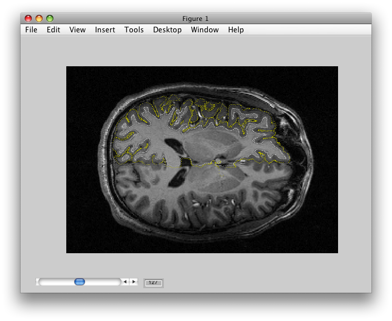
Surfaces start with segmentations. A segmentation refers to segmenting the gray matter from the white matter of the cortex. For example, the image below shows an example of a segmentation generated by SurfRelax:

Note how the yellow dots follow the outer surface of the gray matter and the white dots follow the inner surface of the cortex. How well the segmentation is done is absolutely crucial for how well the surface visualization works. If the segmentation is poor, you might be viewing data not from the gray matter but from the white matter instead. It is thus always a good idea to carefully examine the segmentations that you have generated with outside tools using the flat and surface viewers (see the tutorial for more info on this). If you think you have a bad segmentation (i.e. the yellow and white dots don't follow the outer and inner surfaces of the gray matter), it is a very good idea to go back to your segmentation software and tweak parameters until you get a good segmentation.

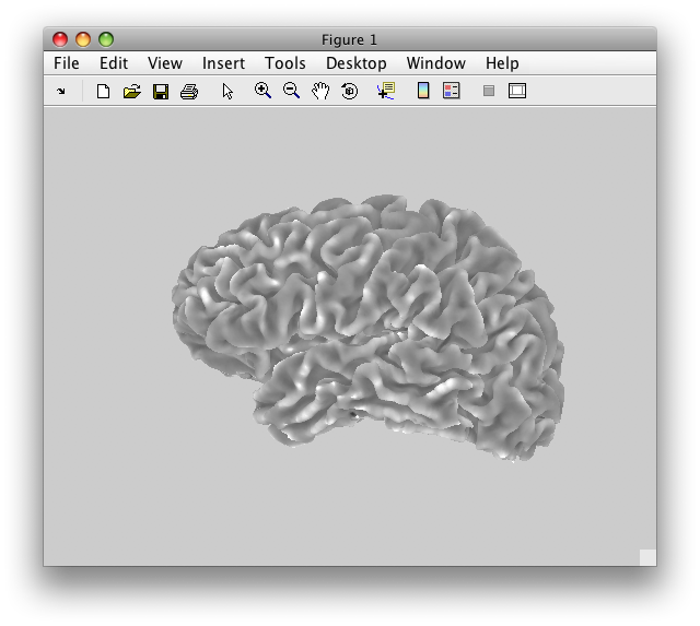
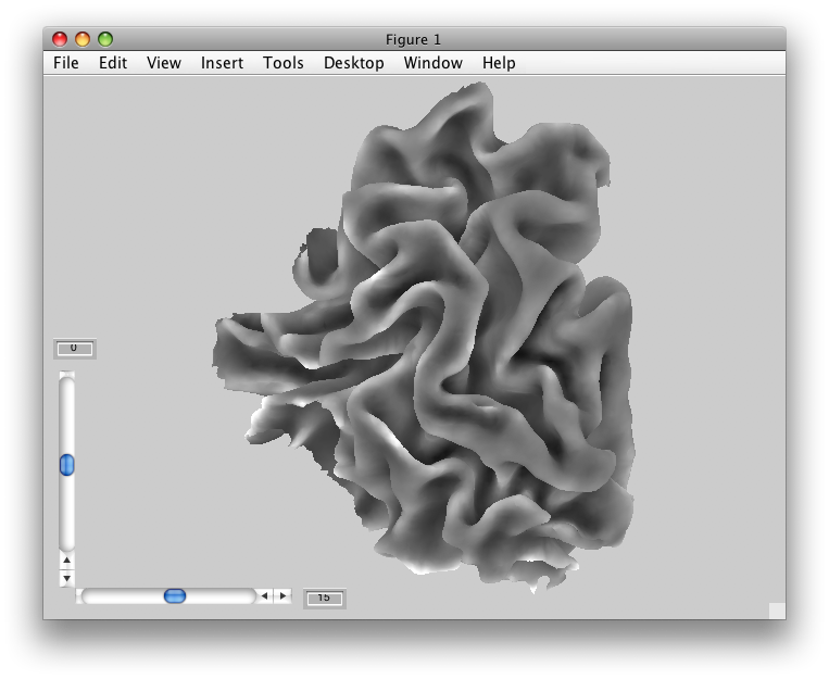
Once a segmentation is done, your surface generation software will generate a 3D surface out of the segmentations. Here is one that SurfRelax created:

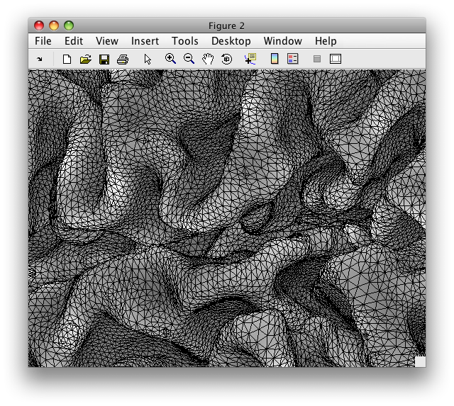
While the image above makes it look like we have a very smooth surface, in actuality we have a surface that is composed of many, many flat little triangles. It is easiest to see this if we look at a zoomed up view of the same surface, and draw the edges of these triangles:

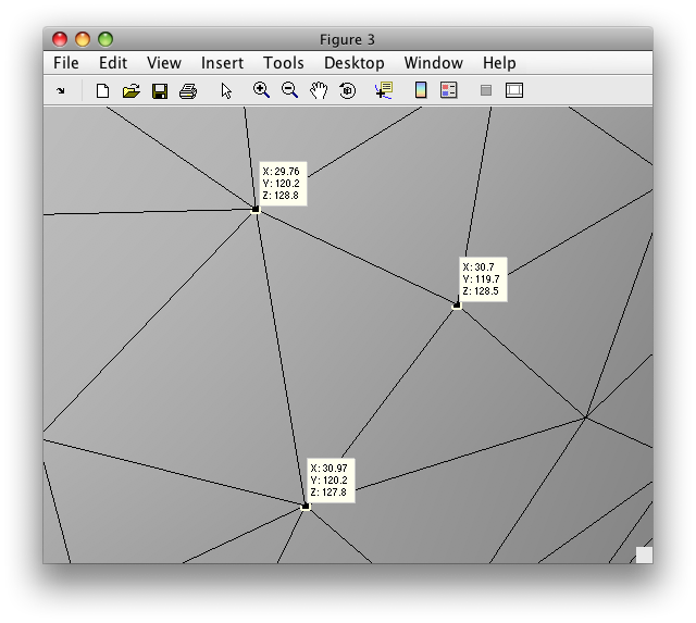
Each of the little triangles you can see are specified by the coordinates of their vertices. To see this, we zoom in a bit further and show you the coordinates of the three vertices of one particular triangle:

Note that the x,y,z coordinates of each vertex is the actual location of that particular vertex in the volume from which the surface was created. That is, in the first image shown above which shows the segmentation as yellow and white dots, each one of those dots is a vertex. The location of the vertex is specified as the coordinates in that 3D volume image. This is important! To be clear, the 3D volume might be an image that is 256x256x176 (for instance). Then the x,y,z coordinates of each vertex is an actual voxel location within that 3D image from where it came from. Note that the x,y,z coordinates can be a fractional number which specifies a location within a voxel.

So, the specification of the surface involves two pieces of information. One is a list of all the vertices x,y,z locations in the 3D volume. The second is a list of which sets of three vertices are connected in a triangle.

So, for example if we load a surface up from the tutorial, you will see that we get both these sets of information:

>> surf = loadSurfOFF('leftInner.off') 
surf = 
    filename: 'leftInner.off'
       Nvtcs: 145596
       Ntris: 291188
      Nedges: 436782
        vtcs: [145596x3 double]
        tris: [291188x3 double]

The vtcs are a list of 145596 vertices (numbered in order) with an x,y and z coordinate. So, for example, the first vertex has a location in the 3D volume that looks like this:

>> surf.vtcs(1,:)
ans =
          74.8006362915039          62.4711685180664          73.3120651245117

And, the triangles are listed as which three vertices (remember the vertices are numbered in order) that are connected to each other. So, for example, the first triangle connects the first three vertices together:

>> surf.tris(1,:)
ans =
     1     2     3

Note that there is a convention to how the vertices are ordered. The convention adopted by SurfRelax is that the vertices are ordered in clockwise order when viewed from the outside. If your segmentation software follows a different convention, then it is possible that flat maps will be shown in the wrong orientation (that is, you need to xy flip them so that right is right and up is up).

There is one final piece of information that is useful for drawing the surfaces. That is what color each vertex is. Typically for our surfaces, we use the curvature. The curvature is what it sounds like, how curved the surface is and in which direction (convex or concave). Technically, we are computing the mean curvature of the surface. We use the function calcCurvature to compute a curvature file which simply is a grayscale value that tells us how to color each vertex in the surface. There are as many values of the curvature as there are vertices. Each triangle of the surface is then colored in such a way that each vertex is colored with its specific curvature value and parts of the triangle in between vertices are interpolated between these colors. If you have done the tutorial, you can load in the computed curvature. We also clip the color values of the curvature, so that it will display nicely.

>> curv = loadVFF('leftCurvature.vff');
>> length(curv)        
ans =
      145596
>> curv(curv<-1.2) = -1.2;curv(curv>1.2) = 1.2;

So now we have all the information that defines the surface: The vertices with their 3D coordinates in the volume, the triangles which specify which vertices are connected together, and the curvature which tells us how to color each vertex. You can easily display a surface like this in Matlab:

>> patch('vertices', surf.vtcs, 'faces', surf.tris,'FaceVertexCData',curv','facecolor','interp','edgecolor','none');
>> colormap(gray);

So, your segmentation and surface generation software (e.g. FreeSurfer or SurfRelax) needs to create two surfaces like the ones described above. It is important to note that the surfaces are in register, in the sense that they have the same number of vertices and triangles. The only difference between the two surfaces is the location of the vertices (either on the pial or gray/white matter boundary).

Any program that can generate the outer and inner surfaces as described above, can be used to generate the types of surfaces that are used in MLR. All you need is to make sure that these two surfaces are in “.off” format, which is a fairly simple format that can be written out of matlab using our function writeOFF.

Note, that SurfRelax uses .off files as it's native format. If you use Free Surfer, you can use the function mlrImportFreeSurfer to convert Free Surfer files to .off. If you are using other software and you read in your surfaces to Matlab, you should be able to write them out in .off format using the function writeOFF.

Now that you understand how surfaces are represented as a set of vertices and triangles, we can explain how MLR uses this information to display your data on a surface.

It's really simple.

The vertices in each surface are the x,y,z location in the 3D volume anatomy from which it was created. MLR using the Nifti Sform matrices of your 3D volume anatomy and the EPI images, can compute the transformation that takes you from the volume anatomy to the corresponding point in the EPI image. We call this the base2scan transformation matrix, and it can be retrieved from MLR using viewGet(v,'base2scan').

So, to color the surface with an overlay, MLR multiplies each vertex coordinate with the base2scan transformation and finds the position in the scan that is associated with that vertex, and then colors that vertex according to the color of the overlay at that position.

Now what is important to understand is that when we display surfaces there are really two different kinds of surfaces that are important. Display surfaces and coordinate surfaces. The coordinate surface is the one just described above. It is the one that tells us where each vertex that we are displaying is in the 3D volume. Often, when we display our data, the display surface will be one and the same as the coordinate surface. But, it doesn't have to be the case. For example, if we have an inflated surface (that is in register with the coordinate surface, i.e. has corresponding vertices and triangles), then the vertices of the inflated surface are in a different location than the coordinate surface (i.e. they are inflated). That way the surface we display is inflated, but the coordinates that are used to get the data come from the right part of the gray matter.

We also keep track of two depths of cortex, the outer and inner layers. That way, when we set the cortical depth slider to 1, we can display the outer display surface (using it's associated outer coordinate surface), and when we set the depth slider to 0, we can display the inner display surface (using it's associated inner coordinate surface). When we set the slider in between 0 and 1, we take an appropriate linear interpolation between the inner and outer surfaces.

So, the first time you want to view a surface in MLR, you can import the surface from the two .off files for the outer and inner surfaces. Use:

File -> Base Anatomy -> Import Surface

Choose the outer (GM) .off file from your volume anatomy folder (which can be set in Edit → Preferences)

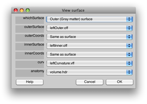
This brings up a GUI that looks like this:

This allows you to select which surfaces to use for what. The outerSurface and innerSurface fields refer to the display surfaces. The outerCoords and innerCoords refer to the coordinate surfaces as explained above. The curv is the curvature and the anatomy file is the 3D anatomy that was used to generate the surface. It is important to specify the anatomy file since it contains the coordinate transform that is used for displaying data on the surface.

The whichSurface field at the top is used to switch what surface is displayed in the viewer while you are selecting files. It does not affect the final surface that is generated for MLR. It is always a good idea to go and inspect the 3D anatomy with the whichSurface selector to make sure that the inner and outer coords are well matched to the location of the inner and outer surface of the gray matter.

Here are two examples of settings used in this dialog:

• Load a folded surface Set both the Outer Surface and the Outer Surface Coordinates to the outer (GM) .off file, and set both the Inner Surface and the Inner Surface Coordinates to the inner (WM) .off file. Note that you always want to have the coordinates be the uninflated surfaces.
• Load an inflated surface To look at an inflated surface, set the Outer Surface to the inflated.off file instead of the outer (GM) .off file. The Outer Surface Coordinates must still be set to the outer (GM) .off file. The Inner Surface and Inner Surface Coordinates should both be set to the inner (WM) .off file. Now, when you move through the cortical depth, you will be moving from inflated to folded as well as from the outer to the inner surface.

Once you have imported a surface, and you are happy with it, then go ahead and save it. The next time you want to view the surface, you can simply open it up as any other Base Anatomy using File/Base Anatomy/Load.

Internally, MLR keeps all the information related to a surface as a combination of a Nifti image and a Matlab base structure. The Nifti image simply contains the curvature image. It is a large 1 dimensional image where each point in the image is the curvature of a single vertex. The matlab base structure contains various information about the anatomy (it is common to all base anatomies) including user settings, and looks like the following:

>> base = viewGet(getMLRView,'base')

base = 

                 clip: [-1.5 1.5]
             coordMap: [1x1 struct]
             curSlice: 1
                 data: [1x145596 double]
                gamma: 1
                  hdr: [1x1 struct]
                 name: 'leftOuter'
    permutationMatrix: [3x3 double]
                range: [-1.5 1.5]
               rotate: 0
     sliceOrientation: 1
            talPoints: []
                 tilt: 0
                 type: 2
              vol2mag: [4x4 double]
              vol2tal: []

Note that the base.type = 2, which means that this base is a surface. The field coordMap contains all the information about the vertices and triangles:

>> base.coordMap

ans = 

                    path: '/Volumes/drobo/data/nyu/surfTutorial/Segmentation'
    innerSurfaceFileName: 'leftInner.off'
     innerCoordsFileName: 'leftInner.off'
    outerSurfaceFileName: 'leftOuter.off'
     outerCoordsFileName: 'leftOuter.off'
            curvFileName: 'leftCurvature.vff'
            anatFileName: 'volume.hdr'
             innerCoords: [4-D double]
               innerVtcs: [145596x3 double]
                    tris: [291188x3 double]
                   outer: 'leftOuter.off'
             outerCoords: [4-D double]
               outerVtcs: [145596x3 double]
                  coords: [4-D double]
                    dims: [256 176 256]
                  rotate: 0

The outerVtcs and innerVtcs are the display vertices. The outerCoords and innerCoords are the coordinate vertices. The tris are the triangles (note that because the inner and outer surfaces are in register, we only need to save one version of the tris). The coords are the current coordinates, which are computed as the linear interpolation between the outer and inner coords depending on how the cortical depth slider works. Also, the names of the files and path are stored in the structure so that when you call the mrSurfViewer from Plots/Surface Viewer, the correct files can be loaded up. If the path of the files has changed, MLR will ask you to specify the new path when you open up mrSurfViewer.

Flat patches are based on the same principles as the surfaces (and are generated from the surfaces), but being 2D are treated somewhat specially by MLR.

A flat patch starts out as some small part of the surface that is cut out:

Then, flattening algorithms can be used to flatten this representation into 2 dimensions. There are different flavors of algorithms that do this, but in general they can be thought of as optimization routines that try to place all the vertices on the same 2D plane, while trying to minimize the amount of distortions caused by the flattening process (i.e. changes in the relative distance between vertices). We have setup MLR to use either the Stanford VISTA mrFlatMesh tools or Surf Relax. The flattened patch ends up looking something like this:

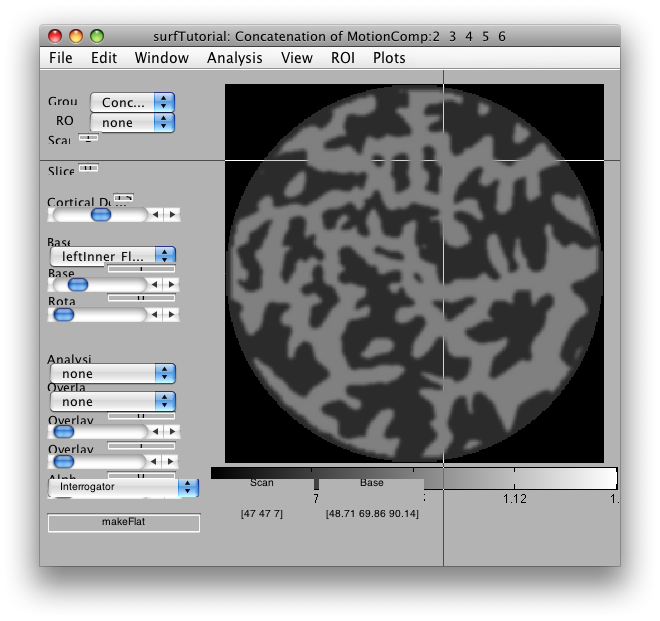
Two things have changed from the previous view. One is that the smooth curvature values have now been thresholded so that there are only two colors being displayed – this is just done to make it look pretty. The second is that the cutout patch is now a 2D image rather than a 3D surface. We have actually changed the 2D flat surface into an image, which can be saved as a Nifti file. The data structure that MLR uses is very similar to that of a surface:

>> base = viewGet(getMLRView,'base') 

base = 

                 clip: [0 1.5]
             coordMap: [1x1 struct]
             curSlice: 1
                 data: [301x301 double]
                gamma: 1
                  hdr: [1x1 struct]
                 name: 'jg_left_occipital'
    permutationMatrix: [3x3 double]
                range: [0 0.75]
               rotate: 63.499996
     sliceOrientation: 1
            talPoints: []
                 tilt: 0
                 type: 1
              vol2mag: []
              vol2tal: []

>> base.coordMap

ans = 

                   path: '/Volumes/CBIV2/Heegerlab/anatomy/jg19710606/jg041001ver2'
           flatFileName: 'jg_left_occipital.off'
    innerCoordsFileName: 'jg_left_WM.off'
    outerCoordsFileName: 'jg_left_GM.off'
           curvFileName: 'jg_left_WM_Curv.vff'
           anatFileName: 'jg041001.hdr'
                 coords: [4-D double]
            innerCoords: [4-D double]
            outerCoords: [4-D double]
                   dims: [176 256 256]

Note a few things from the above. The base.type = 1, which indicates this is a flat map. In the field base.data is the 301×301 image for this particular flat map. It is what we see in the viewer window. There is nothing special about the size 301×301, it just so happens that when we flattened the surface and set it to have a resolution of 2, it turned into a 301×301 sized image. If we had set the resolution to 4, the resolution would be 602×602. Now, any given point on that image is associated with some point in the 3D volume. That is known from the coords field of the base structure. Note the size of this field:

>> size(base.coordMap.coords)
ans =
   301   301     1     3

It has 301×301 because it is the same dimensions as the flat map image. The last 3 is that each point in the 2D image is associated with an x,y,z point from the original 3D volume. The 1 can be ignored (it is a place holder for flat maps with multiple “slices”, but is not being used yet). For example, the point in the center of the flat map (150,150) is associated with the 3D volume coordinate 73.6, 51.6, 95.1:

>> base.coordMap.coords(150,150,1,:)
ans(:,:,1,1) =
          73.6470479050564
ans(:,:,1,2) =
           51.642434868004
ans(:,:,1,3) =
          95.1174479268083

So what MLR does to display the overlay for each point in the 2D image, is to look up its coordinates in the base.coordMap.coords field to get the x,y,z of that point in the 3D anatomy. It then uses the base2scan transformation like for the surfaces to find the point in the scan where that point comes from, and the displays the color of that point in the image according to the overlay that is being displayed.

Note that in the coordMap there are three coordinate fields. The coords, innerCoords and outerCoords. The inner and outer Coords come from the inner and outer coordinate surfaces that were used when generating the flat map and represent where each point on the flat map came from the original surfaces. The coords field itself is a derived field which changes depending on how the cortical depth slider is set. If the slider is set to 1, it is equal to the outerCoords, if the slider is set to 0 it is equal to the innerCoords and if the slider is set in between it is an appropriate linear interpolation between the inner and outer coords.

The easiest way to generate a flat map is to use the Interrogator makeFlat. You can use this interrogator from any base anatomy. To turn it on, go to Plot → Interrogate Overlay. Then, select makeFlat from the drop-down menu at the bottom of the viewer, such that makeFlat appears in the interrogator function text box.

This will allow you to make a flat patch whose center is specified by whatever voxel you click on. A GUI will pop up that has that voxel's coordinates entered as the center point for the flat map. You can specify the radius, the resolution (2 is usually fine), and the method. The method can be either SurfRelax or mrFlatMesh. To use SurfRelax you need to have it installed. mrFlatMesh is available as part of the MLR distribution. Note that SurfRelax sometimes gets stuck making patches. If this happens, choosing a larger radius can help, but you may have to go through many iterations to get it to work. mrFlatMesh always makes a usable patch.

If you are looking at a flat patch, and realize you need the patch to be bigger or recentered, simply click on the voxel you would like to use as the center for the new patch. This will bring up the same GUI as above.

The patches you have created are automatically saved as .off files in the anatomy folder [check if this is the anatomy subfolder of the current MLR directory, or the Anatomy folder that has the original .off files].

Once you have a patch you like, that you are going to want to use again, you should save it as a base anatomy. To do this, you can simply do: File → Base Anatomy → Save, and this will save in the 'anatomy' subfolder of the current mrLoadRet directory.

Alternatively, you can do: File → Base Anatomy → Save As, which will allow you to rename the flat patch, as well as save it in the Anatomy directory for that subject. This makes it easier to re-use the same flat patch for that subject across scanning sessions.

Once you have flat patches that you like that you have saved using File → Base Anatomy → Save/Save As you can simply load them in other sessions.

If you have a flat patch generated outside of MLR (from SurfRelax for instance) you can import it form File → Base Anatomy → Import Flat. This gives you the option to use a higher resolution in recalculating the grid from the .off file. Once you're happy with it, you can save it as a Base Anatomy as described above.

When viewing the mrLoadRet compatible gridded flat patch, you have the option to look at the underlying .off patch using the Flat Viewer, which gives you many nice tools, such as being able to visualize where the patch came from on the cortical surface, being able to overlay it with color codes for medial/lateral and rostral/caudal, etc. To do this, while viewing the flat patch in mrLoadRet, go to Plots → Flat Viewer

Another thing you can do in the Flat Viewer is double-check the segmentation by looking at the 3D anatomy.