Table of Contents
Introduction
The key to understanding analysis of any data including BOLD imaging data is to remember that all analyses are models. One designs and runs an experiment, collects data and then models the results and examines the goodness-of-fit and parameters of the model. If you have a good model of the data, then your goodness-of-fit will be good and you will get fit parameters that can be meaningful interpreted. Models contain multiple assumptions about the processes that generated the data, some of which may not be immediately obvious. Those assumptions may be wrong. And if they are, the results that you obtain may not be meaningful. This is true whether you are doing a simple t-test or fitting a complex non-linear model to your data. So, with that in mind, we will use this tutorial to go through a few commonly used models for analyzing BOLD imaging data.
To make things concrete, we will analyze human cortical BOLD responses to visual stimuli in which we know that neurons in primary visual cortex (V1) will show responses to visual stimuli in a particular location in space called a receptive-field. We will go through the most common ways to look at BOLD imaging data that interrogate these receptive-fields with two types of analyses, an “Event-related analysis” and an “encoding model”. Event-related analyses can be thought of as a trial-triggered average response which assumes that overlaps in response sum linearly. Encoding models can take many shapes and forms, but generally mean that you assume a model that encodes the stimulus (in this case a receptive-field) whose parameters are adjusted to give rise to the response measured in a voxel. For this tutorial, we will use a population receptive-field (pRF) encoding model Dumoulin and Wandell (2008) which has been used extensively to make retinotopic measurements.
Note that this tutorial is meant as a quick and practical introduction to these types of analyses and assumes that you have already learned about the biological processes that give rise to the BOLD signal and some of its basic properties.
Learning goals
After finishing this tutorial, you should be able to…
…compute an event-related analysis of BOLD data to recover the response to a trial or stimulus.
…compute a pRF analysis which allows you to recover the position and size of a visual receptive-field of a voxel.
…know the assumptions (particularly linearity) of each of these models.
Setup
This tutorial is written in Matlab (though there are equivalent instructions in python for the pRF part).
To setup for matlab, you just need to do the following:
- Setup your matlab environment For those working at Stanford you can get an indiviudal license. If that fails, you can try to use the corn server, but we don't recommend that anymore. If you use the corn server, then you do not need to do the rest of these instructions.
- Start matlab
- Get datafiles You can get the data from here. This should download a matlab file to your Downloads folder (if you are on a Mac). To load the data in, you can do:
cd ~/Downloads
load boldmodels
BOLD Response
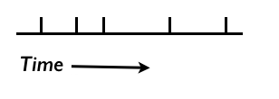
Ok, let's say we do a totally simple experiment in which we flash a visual stimulus at different times and measure the BOLD response in visual cortex. In the diagram below each vertical tick is meant to represent a time at which we flashed the visual stimulus on.
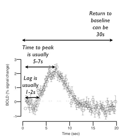
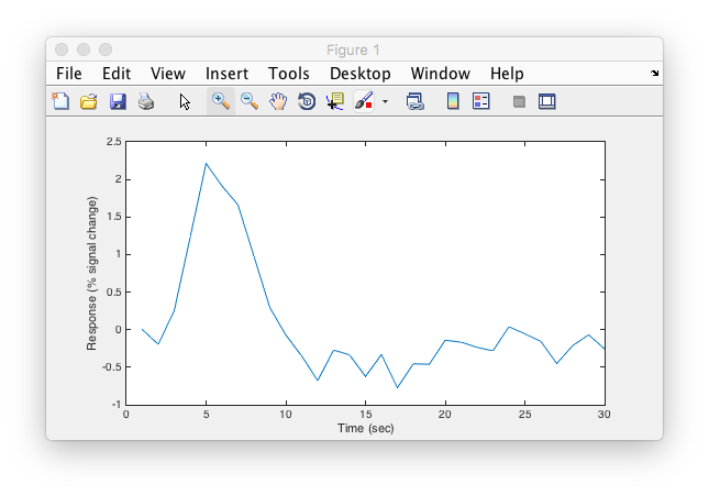
What would we expect the BOLD response to look like? Well, recall, that after brief neural activity, the “hemodynamic impulse response function” typically looks like the following:
The BOLD response is also (approximately) linear in time (see Boynton GM1, Engel SA, Heeger DJ (2012) for an excellent review). What does that mean? It means that it obeys linear superposition - if you know the response to each of two stimuli presented alone, then you can predict the response to the combination of the two stimuli as the sum (or superposition) of the two responses. In this case, the two stimuli would be responses presented at different times which would both be expected to evoke the above hemodynamic response. The response to two stimuli presented in succession would be the sum of the individual responses. So, imagine in your head a hemodynamic response function placed at every vertical tick mark in the stimulus timing diagram above and any overlap in response (when stimuli are closer together than the length of the hemodynamic response) summing together (assume that each tick happens about 5-10 seconds after the last one). Add a little bit of noise to that mental image. Got it? You should be imagining something like the following (Click below to reveal what the expected response is):
Looks like what you got? Good. You've just done a convolution in your head then! That's the linear systems model for a BOLD response and there's pretty good evidence that if you make your stimulus presentation times long enough (a couple of seconds) that the BOLD response is temporally linear (see review cited above). Pretty much every BOLD analysis technique rests on this temporally linear model of BOLD responses!
Event-related analysis
Ok. So, now let's go backwards. Imagine that you have measured that BOLD response time series was and you wanted to know what the average BOLD response was to each stimulus presentation. Well then your model would look something like this:
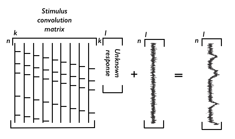
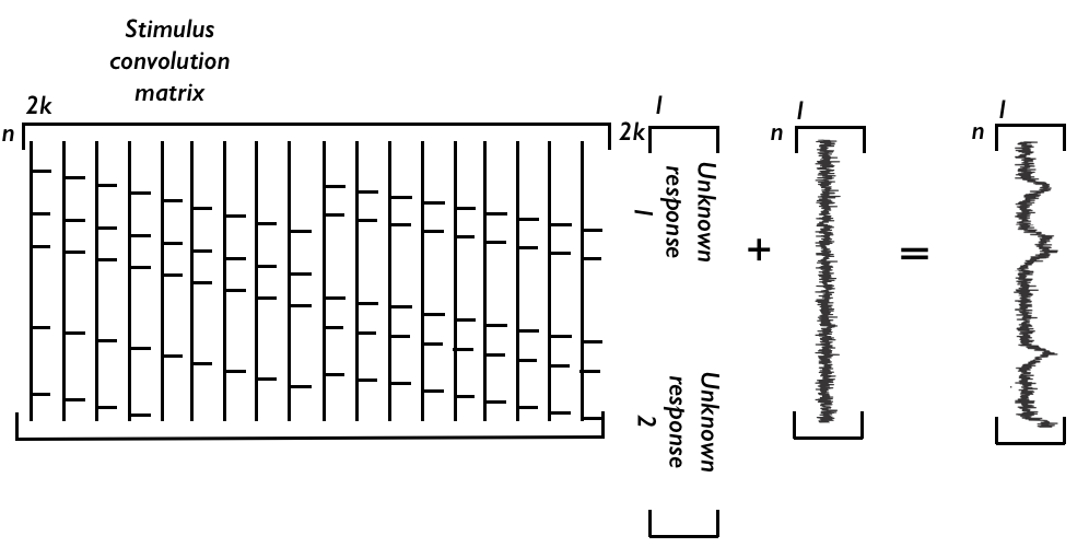
In words, our model is that the stimulus timing convolved with an unknown hemodynamic response plus noise gives the measured bold response. We want to know what that unknown hemodynamic response looks like, so we need to somehow “unconvolve” the stimulus timing from both sides to solve for the hemodynamic response. How is this done? Well, the above can be written in matrix form. It looks like this:
The matrix on the left is just the way that you write down a convolution of the stimulus times with the hemodynamic response. Each column is the stimulus timing shifted downwards one (note that each column as numbers is zeros with ones every time a stimulus happens). Why does this compute a convolution in which response overlaps sum? Try to puzzle through the matrix multiplication by multiplying one row at a time of the convolution matrix with the hemodynamic response to get each time point of the measured BOLD response and you should see that it does the right thing. Make sense? If not, we will go through a concrete example with matlab in a sec, so try to figure it out there. Ok, what about the dimensions? In the above, we have n=number of timepoints in the experiment and k=number of timepoints in estimated response. Note that we have a choice over k - how many time points to compute out the hemodynamic response for. Typically you want to choose k such that you recover the full hemodynamic response, but not too long since every point you estimate will increase the number of unknowns you are solving for, making your estimates worse.
So, how do we solve this? Well, typically one assumes that noise is white (IID - independent at each time point, identically distributed - which is wrong, btw, since BOLD data typically have temporal auto-correlation - that is, timepoints near each other are correlated). But, going with that assumption, this is just a matrix multiplication and you can use the least-squares solution (i.e. solve for the unknown hemodynamic response that minimizes the squared error between the left and right sides of the equation). Note that the noise here isn't something that we are estimating - it is just the left over residual after the model fit. If we have S as the stimulus convolution matrix, h as the unknown response and B the measured response, that's just an equation like:
S x h = B
The least-squares solution is obtained by multiplying both sides by the transpose of S (in matlab notation S'):
S' x S x h = S' x B
Then multiplying by the inverse of S' x S (that's an important matrix, by the way, called the stimulus variance/covariance and can be used to diagnose problems with your design since the more variance in the design gives you more power to estimate parameters - in fact, this inverse of the variance/covariance matrix is used to project residual variance back to get error bars around estimates). That gives us:
h = (S' x S) ^ -1 x S' x B
And that's it, that's an event-related analysis (sometimes people call this deconvolution or finite impulse response estimation). So, how about trying it on real data?
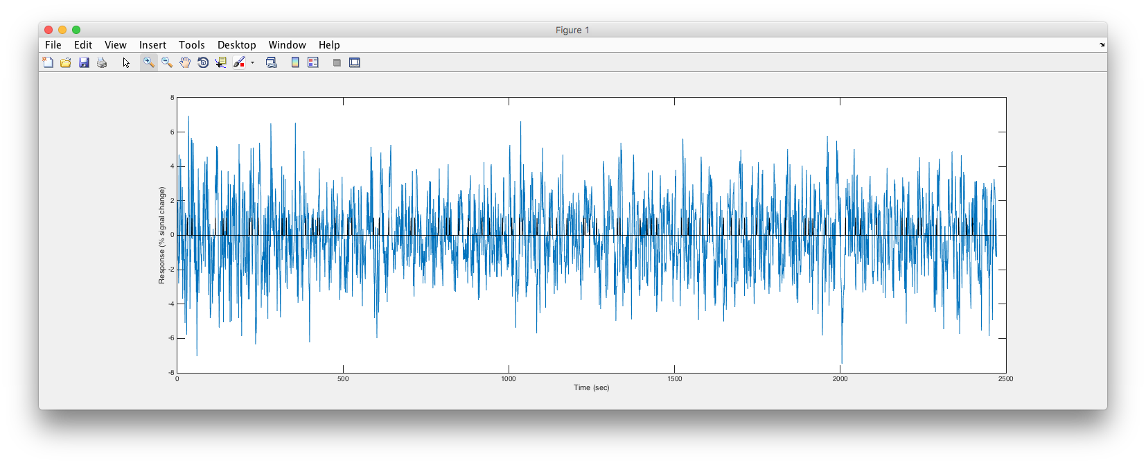
In Matlab, you should have two variables. timeSeries and stimulusTiming. timeSeries is the BOLD response from a single voxel in a part of primary visual cortex. The data were collected every 1s. Typically the data needs to be high-pass filtered to get rid of slow drifts in signals. The time series also has been divided by its mean and multiplied by 100 so that everything is in percent signal change relative to the average pixel intensity. Finally the mean has been subtracted (this is actually really important, since the model we are fitting here doesn't have a term to account for the mean response, so if you don't subtract the mean things won't work!).
Go ahead and plot these two arrays and see what they look like.
Any hint of what the response is? Let's try to form the stimulus-convolution matrix. Each column of the matrix should be a shifted copy of the stimulusTiming array as we discussed above. Let's compute the response out for 30 seconds. So, that means 30 columns (since each data point is 1s).
If you got that right, you should be able to look at a small part of the matrix (say the first 300 rows) and see that the matrix has the slanted line structure that we talked about above. Go ahead and take a look to confirm that.
Ok. Cool. So, now to compute the event-related responses, just plug into the formula from above for getting the least-squares estimate and plot what you get.
Should look like the following:
Easy-peasy. Right? One thing - how good a model is this of the response we measured? Whenever you fit a model you should ask whether you have a statistic that tells you that. One that we have used is to compute the variance accounted for by the event-related model. To do this, you can take the hemodynamic response you estimated and multiply it back through the stimulus convolution matrix. That will form the ideal response as if every trial created exactly the same response and response overlaps summed linearly. That's your model. Subtract that from the time series to get the residual. Now compute r2 as one minus the ratio of the residual variance to the original variance of the time series.
Challenge question
Ok. Challenge question here. The data from above is actually from a paradigm in which we showed a stimulus either in the left or right visual field. Of course we know that primary visual cortex should only respond to a stimulus in the contra-lateral visual field. So, let's say I give you the stimulus time for the times when the stimulus was in the left visual field, and the times at which the stimulus was in the right visual field. You should get a nice response to the contra-lateral stimulus and a flat line for the ipsi-lateral stimulus. Right? But, how do I compute the response for two different stimuli? Well, same way. You just assume that the responses to the two stimuli sum linearly! Try to draw out how to make the matrix equation do that. Be careful of matrix dimensions - make sure they match-up correctly. How would you do it?
Got it? Ok. Then here's your challenge. There's a time series called mysteryTimeSeries. Make the stimulus convolution matrix for stimulusTimingLeft and stimulusTimingRight and compute the response for the mysteryTimeSeries (it will be one long vector with the concatenated responses to the two different types of stimulus).
Which hemisphere did this voxel come from?
General Linear Model
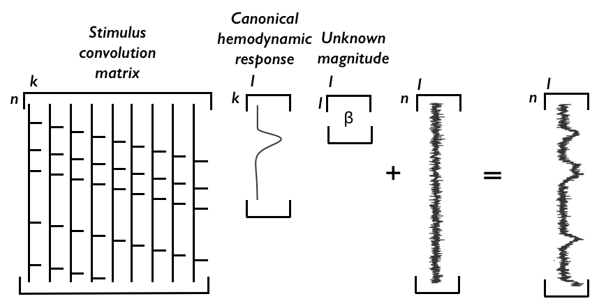
Quick note here is that the event-related analysis is a form of “general linear model” in which the measured responses is modeled as weighted sums of different variables (in this case, different contributions of events from different time points). The event-related analysis shows you something pretty close to a trial-triggered average (assuming that response overlaps sum linearly) so is fairly close to the original data, but can require a lot of data to fit well since you have many unknowns (every time point in the estimated response is an unknown). If you knew the shape of a hemodynamic response function, then you could simplify the computation down to a single number - the magnitude of the evoked response. That would look like the following:
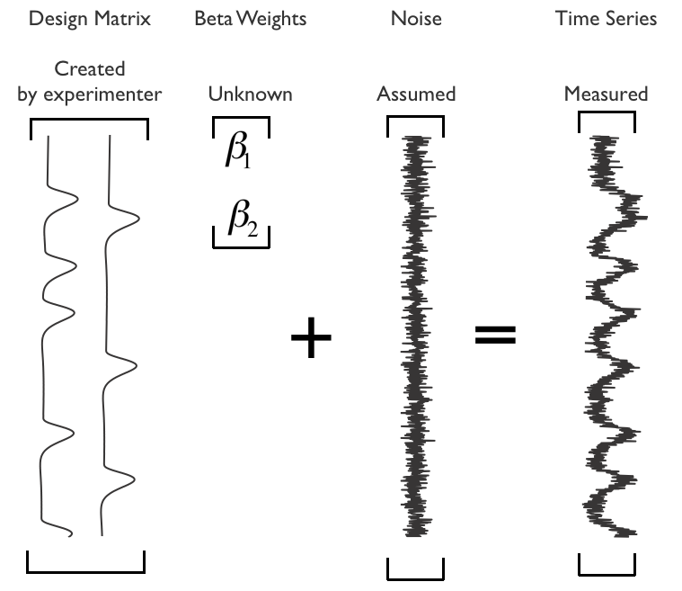
All we have done here is insert a “canoncial” hemodynamic response of unit response (typically you either set the amplitude or the area under the curve to equal one), and now only have to estimate a single number to get the magnitude of response (traditionally this number is called a beta weight). This can be effective because it means there are less unknowns to compute, but can be problematic if the canonical hemodynamic response function you have assumed is wrong. Typically, the convolution is precomputed so that each column of the “design matrix” represents the effect of a different stimulus type (you can also put in other columns to represent things like head motion or linear drift) and a set of beta weights are computed.
The least squares solution for the GLM above is computed in the same way as we did for the event-related analysis.
pRF Encoding model
If we are interested in where visual receptive fields are, we could continue the approach from above by testing stimuli at different locations of the visual field and then computing event-related responses. But, there is a much better way to do this. That takes us to the idea of encoding models!
Encoding models of various forms have become a powerful tool for analyzing functional imaging data because they can build on knowledge of how different parts of the brain respond to stimuli. A simple, but really useful encoding model is the population receptive field model (see Dumoulin and Wandell (2008) that is used routinely to make topographic maps of visual areas in human visual cortex.
First, take a few minutes to go through Dan Birman's excellent conceptual introduction to the population receptive field.
Got the idea? Cool. A few key points to take away from this. The encoding models are useful because they allow you to predict what responses will be like to stimuli that you have never presented before, which also allows you to decoding - given a response what stimulus caused this response? The idea is very general and powerful - while we do this for a simple receptive field, an encoding model can be anything - could be a sophisticated receptive field model selective for different visual features, could be the output of a deep convolutional network, or a model for language.
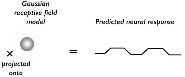
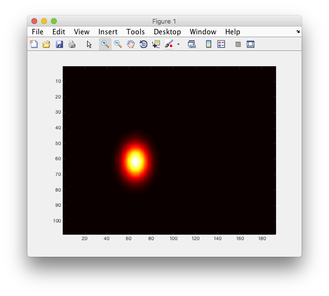
So, the basic idea of any encoding model is to make a model that, well, encodes the stimulus. This model is a hypothesis for how you think the area responds. For visual cortex, the simplest model is that neurons respond to a localized position of space, i.e. has a receptive field. As the BOLD measurement will pick up hemodynamic changes related to a population of neurons, the hypothesis will be that there is a “population receptive field” associated with each voxel. That looks something like the following:
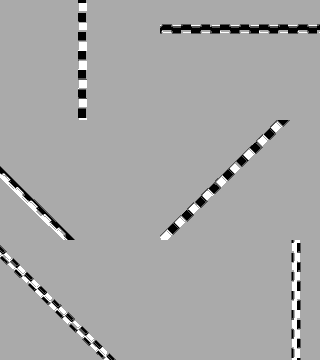
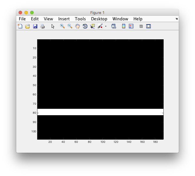
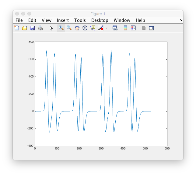
Where the stimulus is high-contrast bars moving through the visual field (while the subject fixates at a single position in the center of the screen) and the population receptive field encoding model is a gaussian. The predicted response is simply the projection of the stimulus on to the receptive field - which means that every time frame of the visual stimulus you multiply the visual stimulus with the gaussian receptive field and sum that all up to get the predicted neural response at that time. With that predicted neural response in hand, you can get a prediction for the BOLD response similar to what we did with the event-related response:
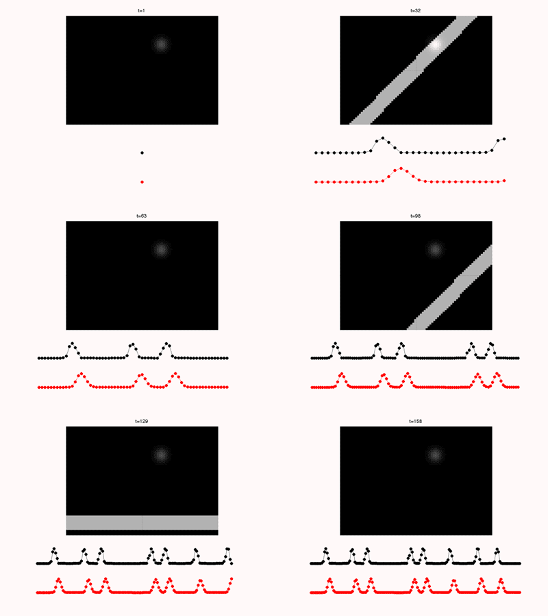
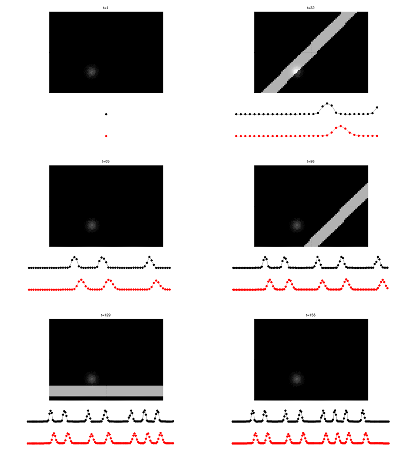
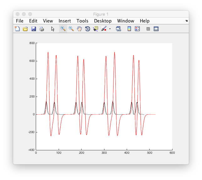
That is, we simply convolve with a hemodynamic response. That's it. That's a prediction for the voxel response for a given receptive field at a particular location and width. Of course, if the receptive field is in a different location - or has a different size - it will predict a different BOLD response. Here are two different receptive fields with the neural prediction in black and the BOLD prediction in red. You should be able to see that they make different predictions as the bar stimulus crosses their receptive fields at different times.
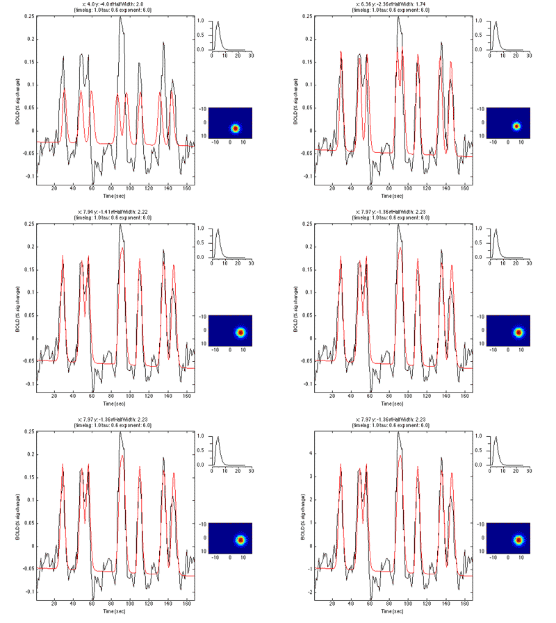
So, to fit the pRF encoding model, you just look for the receptive field location and size that best predicts the BOLD measurement you made at each voxel. You can assume a canonical hemodynamic response function or you can allow that to change to best predict the data as well. Here's a non-linear fitting algorithm searching for the best parameters for a particular voxel. Black is the measured time series, red is the fit and the lower right shows you the population receptive field that gives that prediction.
Now, we'll try and fit this model to real data. Note that we will just do a very rough fit using a grid search so that you get the idea of how the fit is done. For those interested, a more thorough tutorial in which includes non-linear fitting, projected data onto cortical surfaces and decoding is available here. For a tutorial on how to do this analysis and mark retiotopic boundaries for your own data using the GUI in mrTools, see here.
Compute the model neural response
Examine the stimulus matrix
Let's start by just taking a look at the stimulus that was presented to the subject. Remember the subject was looking at the center of the screen where there was a fixation cross on which they had to perform a task (just to keep their attentional state and fixation under control) and bars moving in different directions were shown. Each frame of the image is stored as a 2D matrix that has the pixel values for each position on the screen. For this purpose, the matrix just contains 0's and 1's. Each of these 2D frames are stacked into a 3D matrix where the third dimension is time.
So they just look like images, let's go ahead and display an arbitrary image, say the 36th image, and see what we get.
Now that you can display the image, you might want to go ahead and look at the whole sequence. You can write a for loop and display each image at a time and see what it looks like.
Good, you should have seen a bar move in various directions across the screen. That was what was shown to the subject. Run again, and count how many times a bar crossed the screen - we'll need that number as a consistency check in a following section!
Compute a gaussian receptive field
Now we need to make our encoding model. In this case it is a simple gaussian receptive field. Let's start by making an arbitrary one at the location (-12, -3) degrees (i.e. 12 degrees to the left and 3 degrees below center) We also need to set the size of the receptive field, let's do one that has a standard deviation of 3 degrees. So, first, your going need to know the equation of a gaussian, right?
The x and y coordinates of every point of the stimulus image is in stimX and stimY, so using the 2D equation with those input points, you should be able to compute the gaussian receptive field.
Compute the model neural response
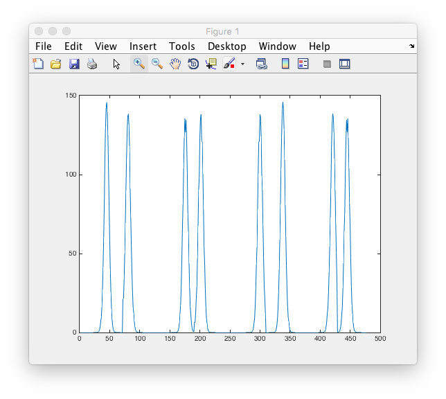
Now that we have the receptive field and the stimulus, it's time to compute the expected “neural response”. The amount of overlap between the stimulus and the receptive will govern the neural response. (For our purposes we won't consider any of the dynamics of neural responses themselves - e.g. transients, adaptation, offset responses, etc etc) To compute the overlap, we just take a point by point multiplication of the stimulus image with the receptive fields and sum across all points. You should now try to compute that for every time point in the stimulus image.
How many peaks in this simulated neural response do you see? Does it match the number of times there was a bar moving across the visual field that you counted above?
Compute the model BOLD response
Now we have to convert this model neural response into a model BOLD response. The model that we use for this is that the BOLD response is a convolution of a canonical hemodynamic response function with the neural response. So, go ahead and compute the convolution of the model neural response with the canonical hemodynamic response function (we have provided one in the variable called canonical
Ok. Sanity check (always good to check that things are making sense as you go along as much as possible). Plot the neural response on the same graph as the bold response and see if they make sense. In particular, the bold response should start after the neural response and last longer, right?
Ok. Looks good? What about at the very end. Do you notice that the BOLD response lasts longer than the neural response? That's because the conv command returns a vector longer than the original response. We don't want that last piece, so remove it from the bold model response (otherwise, dimensions won't match for the calculations we do later). Also, let's take the transpose of this modelBoldResponse (also important for matching dimensions up later)
Compare the model to measured responses
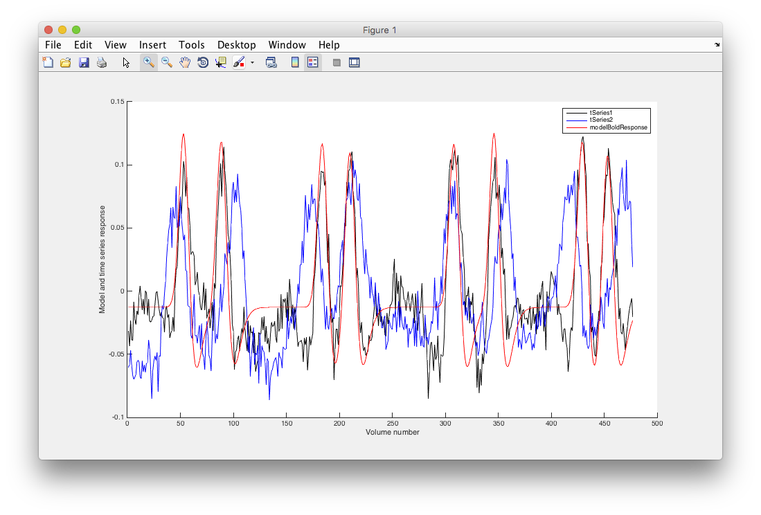
Ok. So, we can compute the model BOLD response for a specific receptive field - now we want to know how to compare that to measured responses. We're going to use the time-point by time-point correlation between the model and the measured responses. Correlation is a nice measure to work with, since it isn't affected by the magnitude of responses. Remember that we haven't really done anything to make the units of the model match the units of response (look back at the units you have for the model BOLD response - typical BOLD responses are about 1 or 2% signal change - is that the size of the fluctuations you have in the model? (no. right!). We'll get back to that in a bit below, but here we'll just ignore the whole issue by using correlation. Ok, we have two actual time series for you to work with tSeries1 and tSeries2 (they were measured from a subject viewing the stimuli). Go ahead and compute the correlation between these time series and the measured bold response from above. What do you get? For which tSeries is this model rf a good model for?
Ok. Let's confirm that visually, by plotting the model and the time series together and see that they match. Now, we have to worry a little about the magnitudes which are going to be different between the model and the actual bold responses. Let's handle that by finding that scale factor. How do we do that (hint - what if I call that scale factor a “beta weight”?). Also, since our time series have the mean subtracted off, we need to subtract the mean off of the model bold response as well (do that first and then compute the scale factor) - general maxim here - if you do something to your data, you need to do the same thing to the model.
So, should be a great match for tSeries1 and a pretty bad match for tSeries2.
One thing about the correlation values. They are a measure of goodness-of-fit. If you square the value then it is mathematically equivalent to the r2 value we calculated above for the event-related model. Really? Check it. Compute the r^2 like we did above. Compute the ratio of the residual variance (subtract the model from the time series) to the original variance. r2 is one minus that ratio. Is that the same as the correlation?
Come out the same? Math. Kinda amazing isn't it. Anyway, this is super important because if your fit is bad (in this case low correlation) then the parameters you fit cannot be interpreted (i.e. the x, y and std of the population receptive field)! So, always (whether you are doing an encoding model or a GLM or whatever) check goodness of fit before trying to extrapolate anything from what parameters you got. To use technical terms, if goodness-of-fit is crap then your parameter estimates will be crap too.
Challenge question
Ok, so of course the example above for tSeries1 was totally cooked - I gave you the parameters that would pretty closely match the response. How can we find the best parameters for tSeries2 (and in general any time series for which we don't know what the receptive field parameters are). After all, that's the whole goal of what we are doing right? To figure out what the receptive field model is that best explains the responses of each voxel. We'll do a quick and dirty way to get close to the right parameters by doing a grid search. What's a grid search? It's just forming a grid of parameters and testing to see which model parameters on this grid give a model response that best fits the voxel. In this case, our grid will be over x and y position of the receptive field and the width (standard deviation). Let's try x and y from -15 to 15 degrees in steps of 1 and standard deviations from 1 to 5 in steps of 1. If you iterate over all combinations of these parameters, compute predicted model responses and compare the correlation with tSeries2, you should be able to figure out the best receptive field for tSeries2!
What are the best receptive field parameters for tSeries2?
