Table of Contents
The following are some introductory lines to the functionality of the mrLoadRet-4.5 Graphic User Interface. All options in this section will either generate a .mat file, modify mrSESSION.mat or the .img files.
File Menu
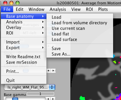
Look in the file menu for functions that let you load / save anatomy files, analyses, ROIs and so on. There are also functions that let you print the currently displayed image, import / export data, ROIs, write out information about the session in a Readme.txt file, and quit the current session of mrLoadRet.
Base Anatomy
- Load: Select an anatomy file on which overlays will be rendered. Normally, this will be your inplane anatomy file which was collected during the scanning session at the same slice locations as your functional data.
- Load from volume directory; Select a volume anatomy file on which overlays will be rendered. By default, the file dialog window opens in the volumeDirectory folder specified in your preferences. Make sure that the qform and sform matrices of the file you select are correct. Normally, you will use the volume anatomy file that was used as the target in your alignment steps (see mrAlign documentation).
- Use current scan Lets you use the current functional scan as the background image. You will be prompted to select a time point from the 4D volume; the first frame in the sequence is 1. If you select time point '0', the mean 3D image across time will be used.
- Load flat Load flat patches created by the steps described in the
- Load Surface Load OFF surfaces created with TFI/SurfRelax. You will be prompted for an outer surface filename. Provide the gray matter (GM) surface from one subject/hemisphere. You will then be prompted to select the matching inner surface (white matter, WM), curvature, and anatomy file. See documentation for mrSurfaceViewer for more details.
- Save Save the currently used anatomy image with a default filename
- Save As… Save the currently used anatomy image and specify a filename
Analysis
- Load Load an analysis that was computed and saved earlier. Standard analyses that can be created by functions accessible in the GUI Analysis menu are Time Series Statistics (e.g. mean, median, across time), Correlation Analysis (standard Fourier-based analysis), Event related analysis, and GLM analysis (generalized linear models to produce statistical parametric maps).
- Save Save the currently selected analysis.
- Save All Save all analysis that have been opened in this session.
Overlay
ROI
Import
- Group
- Time Series
- Overlay
Export
- Anatomy
- Time Series
- Overlay: This function exports the current overlay into a NIFTI file. If a flat map is loaded, the user is asked how many different depths should sample the cortex. If she selects 10 for example, and the flat maps are 384 by 384, the flat map will be exported as a 384*384*10 volume, and each slice will be a different cortical depth.
- ROI
- Image
Write Readme.txt
Save mrSession
Quit
Edit Menu
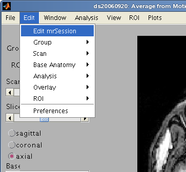
Edit mrSession
Edit details of the scanning session such as a description, the subject id, operator, magnet and pulse sequence. Those were usually when running mrInitRet or mrInit.
Group
Manipulate groups (such as Raw, MotionComp, and Averages
- New Group - create a new group
- Delete Group - delete an existing group, e.g. if you realize that there were some mistakes in averaging across scans, you can delete the group Averages. The function will clean up the appropriate entries in the view variable that goes along with your session.
- Edit Group - This allows you to edit details for each scan in a Group: the scan description, the total number of frames and the junk frames (also called 'dummies') at the beginning of each scan that get disregarded in any analysis.
- Info - show information about each scan in each the current group. For the Average group, this will also show you which files contributed to each average. This is quite an important tool for debugging and checking your analyses.
Scan
Base Anatomy
Analysis
Overlay
- Edit Overlay
- alphaOverlayExponent: this value can be positive or negative. alphaOverlayExponent specifies how much the alphaOverlay masks the selected overlay. With positive value, low values in the alphaOverlay mask more than high values. With a negative exponent, it's the reverse. This is useful for masking overlays with p-value overlays (you want high values to mask more).
ROI
Preferences
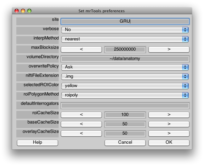
Edit important preferences that affect the overall behavior of mrLoadRet. You will see a menu like the following:
| preference | value |
|---|---|
| Site | (e.g. NYU, RIKEN, RHUL, Nottingham, …) |
| verbose | Yes if you want to have messages and waitbars displayed as dialogs, No to have information printed to the terminal |
| interpMethod | Type of interpolation to use. Normally this is set to nearest for nearest neighbor interpolation – on a flat map you will be able to see a crystalline pattern of how the voxels are getting warped. If you prefer a smoother looking overlay, try setting this to linear |
| maxBlocksize | Size of chunks of data to analyze at a time. If you are running out of memory, set lower. A good starting point is 250000000. If you are using 64 bit Matlab (there is a beta which works with mrLoadRet for Mac OS X), set this to a very high number. |
| volumeDirectory | The directory to default to when you load base anatomies from the VOlume directory |
| overwritePolicy | Method to use when analysis is going to overwrite an existing file |
| niftiFileExtension | Nifti file extension, usually .img but can be set to single file .nii |
| selectedROIColor | What color to use to draw the selected ROI. |
| roiPolygonMethod | Method used to create ROI polygons. The default roipoly function calls the line drawing function which can be very slow if you have already drawn a buch of lines (i.e. have some ROIs displaying). If you choose getpts instead, you will not have the lines drawn between points as you draw the ROI, but it will be much faster. getptsNoDoubleClick is similar to getpts but instead of double-click to end the selection you hit the return key (on some machines Matlab''s idea of what constitutes a double-click can be very slow) |
| roiCacheSize | Size of ROI cache, usually 100. |
| baseCacheSize | Size of base image cache. Set to the number of base slices you want to be able to quickly view |
| overlayCacheSize | Size of overlay image cache. Set to the number of base slices you want to be able to quickly view |
| roiContourWidth | this specifies the linewidth with which to draw the ROI. I find that, depending on the type of base anatomy, I find a value of 2 looks better/worse than a value of 1 (the default) |
Window Menu
New Window
Open up a new window, if you want to e.g. look at the same data set in the coronal and sagittal views simultaneously
New Graph Window
Open up a new graphing window, into which results from new calls to the interrogator functions or functions form the Plots menu get rendered.
Analysis Menu
- Motion Compensation For more info see: Motion Compensation.
- Average Time Series For more info see: Average Time Series
- Concatenate Time Series For more info see: Concatenate Time Series
- Time Series Statistics For more info see: Time Series Statistics
- Correlation Analysis For more info see: Correlation Analysis
- Event Related Analysis For more info see: Event Related Analysis
- GLM Analysis For more info see: GLM Analysis
View Menu
ROI Menu
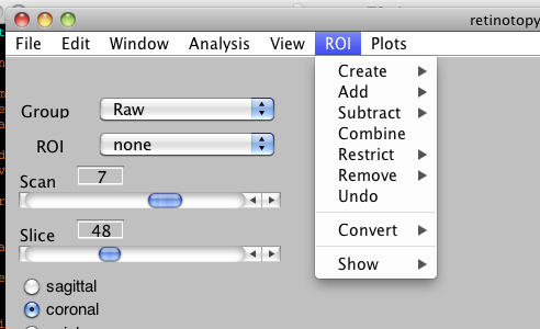
Create:
- Contiguous Voxels (⌘C): Selecting this submenu will create a new ROI and transform the cursor into a selection cross. The user then has to select a voxel that is not masked out in the overlay. The function will select all the voxels that are contiguous to this voxel and that are not masked out, across all the slices (3D contiguous ROI), and add it to the new ROI. The masking depends on the clip values of all the overlays of the current analysis.
Add
- Contiguous Voxels (⌘B): Same as Contiguous Voxels (⌘C) in the Create menu, but adds the contiguous regions to the current ROI
Subtract
- Contiguous Voxels (⌘Y): Same as Contiguous Voxels (⌘C) in the Create menu, but subtracts the contiguous region from the current ROI
Combine
Restrict
Remove
Undo
Convert
- ConvertCoordinates: Lists all the loaded ROIs. Attempts to identify in which coordinates system they are in (e.g., current base, or any other base that is loaded in the view). Then the user can choose to convert the ROIs into the current scan coordinate system, the current base coordinate system, or into any loaded base coordinate system; the user can also choose to adopt their xform.
- This feature is useful in several cases:
- 1: ROIs are created in the coordinate system of the base anatomy that is loaded when the ROI is created. But there are cases where you need the ROI to be in a different system (e.g., if it has been created in low resolution and you want it in high resolution, or if it has been created on a flat map, but you need it in scan coordinates).
- 2: The 'adopt xform' feature is useful when the alignment of the scan to the base has changed. If you want to keep the same ROIs, you can keep the same coordinates (so you don't have to redraw them), but you need to change the xform.
Show
Plots Menu
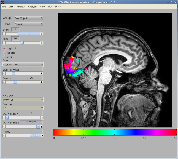
The main GUI window
Overlay Min/Max sliders
The “overlay min” and “max” sliders determine the range of values in the current overlay that are displayed on top of the base anatomy (with the current overlay colormap).
- if maxClip > minClip: (the usual!) display everything on the interval [ minClip, maxClip ]
- if minClip == maxClip: make overlay transparent, display interval is empty
- if maxClip < minClip: assume that user wants to show values more extreme that minClip and maxClip. That is, show all vals < minClip, vals > maxClip (This is useful for displaying e.g. extreme values in two-tailed t- or z-stats).
Note, that
- each overlay in the current analysis contributes to what's shown: multiple selections are combined by a logical intersection.
- the opacity of the selected overlay is further determined by the alpha value on the Alpha slider (or if an alphaOverlay is selected in Edit→Overlay→Edit Overlay).
On the new GUI (see GLM version 2) the controls are similar and are set as follows:
Thresholds and Visibility of voxels: The thresholds that are being used for each clipping overlay are set by the combination of Min/Max sliders and boxes, but can also be controlled through the Edit→Overlay→Edit Overlay window. These thresholds determine whether particular voxels are being displayed as part of the overlay color map or not, but in addition the (alpha) transparency for each voxel can also be controlled. This might be useful if you want to emphasize data with higher statistical significance values.
The overall transparency of the overlay controlled is by the Alpha slider, but the voxel-wise alpha transparency is determined by the alphaOverlay (to get info about the current overlay: Edit→Overlay→Info, to change it, select a different alphaOverlay after Edit→Overlay→Edit Overlay).
