Table of Contents
Event Related Tutorial (scripting)
This shows you had to do all the analysis form the Event Related Tutorial without the GUI. Note that you may also want to set your verbose setting in Edit/Preferences to 'No' so that all messages and waitbars get printed out at the command line rather that in a dialog.
Overview
- Download the tutorial files
- Concatenate scans together
- Set stimfiles
- Run event-related analysis
- Extracting data
1. Download
You can download the tutorial files from:
Note that this is a rather large file. Approximately 300MB.
The files are provided as a tar/zip file. In Mac OS X you should be able to just click to open the files in the Finder. Otherwise, you can go to a terminal and do:
gunzip erTutorial.tar.gz
tar xvf erTutorial.tar
We assume that you have mrTools running on your system.
2. Concatenate
Start matlab and cd into the erTutorial directory:
cd erTutorial
We will concatenate the scans from the motion group together:
v = newView;
v = viewSet(v,'curGroup','MotionComp');
nScans = viewGet(v,'nScans');
[v params] = concatTSeries(v,[],'justGetParams=1','defaultParams=1','scanList',[1:nScans]);
At this point, the params should look like:
  >> params

params =

                     groupName: 'MotionComp'
                  newGroupName: 'Concatenation'
                   description: 'Concatenation of MotionComp:1  2  3  4  5'
                    filterType: 1
                  filterCutoff: 0.01
                 percentSignal: 1
          projectOutMeanVector: 0
                     paramInfo: {1x7 cell}
                      scanList: [1 2 3 4 5]
                          warp: 0
              warpInterpMethod: 'nearest'
    projectOutMeanVectorParams: [1x1 struct]
                   tseriesFile: {1x5 cell}
We could change any of the parameters that we want at this point, but there is no need, so we will just start the concatenation here:
v = concatTSeries(v,params);
3. Set stimfiles
Here, we write a snippet of code to set all the stimfiles:
nScans = viewGet(v,'nScans','Raw');
for iScan = 1:nScans
  stimfilename = sprintf('stimvol%02i.mat',iScan);
  viewSet(v,'stimfilename',stimfilename,iScan,'Raw');
end
And then check to see if it looks correct
>> groupInfo('Raw')
1: directions/coherences
   Filename: 11+cbi_ep2d_bold_recon.img GroupName: Raw
   StimFilename: /Volumes/drobo/data/nyu/erTutorial/Etc/stimvol01.mat
   junkFrames=[0] totalJunkedFrames=[0]
   voxelSize=[3.0 3.0 3.0] TR=1.2000 Dims: [64 64 22] Volumes=375
2: directions/coherences
   Filename: 12+cbi_ep2d_bold_recon.img GroupName: Raw
   StimFilename: /Volumes/drobo/data/nyu/erTutorial/Etc/stimvol02.mat
   junkFrames=[0] totalJunkedFrames=[0]
   voxelSize=[3.0 3.0 3.0] TR=1.2000 Dims: [64 64 22] Volumes=375
3: directions/coherences
   Filename: 13+cbi_ep2d_bold_recon.img GroupName: Raw
   StimFilename: /Volumes/drobo/data/nyu/erTutorial/Etc/stimvol03.mat
   junkFrames=[0] totalJunkedFrames=[0]
   voxelSize=[3.0 3.0 3.0] TR=1.2000 Dims: [64 64 22] Volumes=375
4: directions/coherences
   Filename: 14+cbi_ep2d_bold_recon.img GroupName: Raw
   StimFilename: /Volumes/drobo/data/nyu/erTutorial/Etc/stimvol04.mat
   junkFrames=[0] totalJunkedFrames=[0]
   voxelSize=[3.0 3.0 3.0] TR=1.2000 Dims: [64 64 22] Volumes=375
5: directions/coherences
   Filename: 15+cbi_ep2d_bold_recon.img GroupName: Raw
   StimFilename: /Volumes/drobo/data/nyu/erTutorial/Etc/stimvol05.mat
   junkFrames=[0] totalJunkedFrames=[0]
   voxelSize=[3.0 3.0 3.0] TR=1.2000 Dims: [64 64 22] Volumes=375
4. Event Related Analysis
Now, we are ready to run the event related analysis.
v = viewSet(v,'curGroup','Concatenation');
[v params] = eventRelated(v,[],'justGetParams=1','defaultParams=1','scanList=1');
Let's set the applyFiltering parameter:
params.applyFiltering = 1;
And run it
eventRelated(v,params);
That's it. To view the analysis, start up mrLoadRet, switch to the Concatenation group and load the erAnal analysis using File/Analysis/Load.
5. Extracting data
Single voxel results
You can also analyze the event-related data in your own programs, by retrieving the outcome of the analysis from a view variable. Start with a new view:
v = newView;
Switch to the last scan in the concatenation group
v = viewSet(v,'curGroup','Concatenation');
nScans = viewGet(v,'nScans');
v = viewSet(v,'curScan',nScans);
Load the event related analysis:
v = loadAnalysis(v,'erAnal/erAnal');
Now get the “d” structure. “d” stands for data and it holds the outcome of the event-related analysis for the scan:
d = viewGet(v,'d');
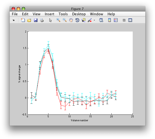
The field ehdr holds the Estimated HemoDynamic Response and the field ehdrste holds the standard error of that response. You could plot the three responses for the voxel [41 46 8], by doing:
figure; hold on;
plot(squeeze(d.ehdr(41,46,8,1,:)),'k');
plot(squeeze(d.ehdr(41,46,8,2,:)),'r');
plot(squeeze(d.ehdr(41,46,8,3,:)),'c');
Or, plot them with error bars:
figure; hold on;
errorbar(1:d.hdrlen,squeeze(d.ehdr(41,46,8,1,:)),squeeze(d.ehdrste(41,46,8,1,:)),'k');
errorbar(1:d.hdrlen,squeeze(d.ehdr(41,46,8,2,:)),squeeze(d.ehdrste(41,46,8,2,:)),'r');
errorbar(1:d.hdrlen,squeeze(d.ehdr(41,46,8,3,:)),squeeze(d.ehdrste(41,46,8,3,:)),'c');
You should see something like this:
You can also get the r2 values, by getting it from the overlay
r2 = viewGet(v,'overlayData',nScans);
The voxel we just plotted above [41 46 8] has an r2 of 0.42 (i.e. 42% of the variance accounted for):
  >> r2(41,48,8)
ans =
      0.06366594
ROI results
You can also recalculate the event-related analysis for an ROI. This is useful to do so that you can get error bars that represent the error over repeats of the stimulus. Continue with the open view we were just using and load the l_mt ROI and its time series:
l_mt = loadROITSeries(v,'l_mt');
Now, let's be a little bit fancy and select only voxels that meet a certain r2 cutoff. It is convenient to start by converting the scan coordinates of the ROI to linear coordinates:
scanDims = viewGet(v,'scanDims');
l_mt.linearScanCoords = sub2ind(scanDims,l_mt.scanCoords(1,:),l_mt.scanCoords(2,:),l_mt.scanCoords(3,:));
now get the r2 values for those voxels:
nScans = viewGet(v,'nScans');
r2 = viewGet(v,'overlayData',nScans);
l_mt.r2 = r2(l_mt.linearScanCoords);
Now, let's make an average time series for all the voxels in the l_mt ROI that have an r2 greater than 0.2
tSeries = mean(l_mt.tSeries(l_mt.r2>0.2,:));
OK. Let's setup to re-run the event-related analysis on this average time series. First we get the “stimvols” which is a cell array of arrays that specifies on what volume each stimulus occurred:
stimvol = getStimvol(v);
Then get the number of stimulus types (each array in the stimvol is for a different stimulus type – in this case a different direction of motion):
nhdr = length(stimvol);
Let's decide on the hdrlen. This is the number of volumes to calculate the deconvolution for:
hdrlen = 20;
And make a stimulus convolution matrix out of the stimvols. Note that this function handles the run boundaries correctly when making the convolution matrix. The 1 specifies to apply the same filtering to the columns of the convolution matrix as was used in concatTSeries.
scm = makescm(v,hdrlen,1,stimvol);
Now run the deconvolution on the mean time series
d = getr2timecourse(tSeries,nhdr,hdrlen,scm,viewGet(v,'framePeriod'));
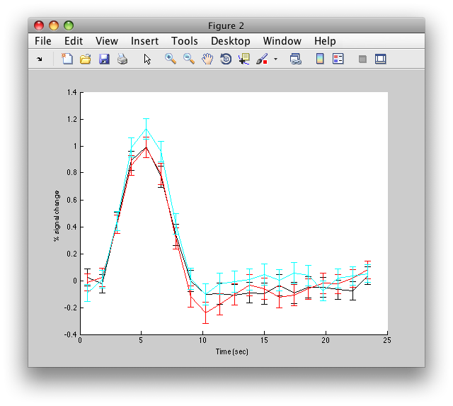
and plot the results
figure; hold on
errorbar(d.time,d.ehdr(1,:),d.ehdrste(1,:),'k');
errorbar(d.time,d.ehdr(2,:),d.ehdrste(2,:),'r');
errorbar(d.time,d.ehdr(3,:),d.ehdrste(3,:),'c');
And you should see something like this:
Note that the error-bars here are over the number of repeats of the stimulus and not over the number of voxels (which are not independent of each other).

