Table of Contents
GLM Tutorial
This tutorial shows you how to run a single-subject GLM analysis with mrLoadRet. The General(ized) Linear Model is commonly used for fMRI data analysis. Basically it is an analysis in which you specify a set of factors that you think will have influenced the time series of your fMRI data and assume that these factors all sum linearly with an unknown weighting (i.e. beta weight) for each voxel. Each factor is really just a vector of 1's and 0's specifying when an event of a particular type happened - for example the presentation of a face stimulus. These are convolved with a hemodynamic response function (typically a canonical form, but can be estimated from data) and put into the columns of a matrix called the design matrix. Then the best beta weights (in a least-squares sense) of each column of the matrix that after summing gives the time series are computed. These beta weights can be displayed, statistics calculated for their significance (i.e. telling you whether the response of a particular voxel is significantly modulated (+ or -) by a factor like the presentation of a face). Or more complex analysis can look at different linear combinations of beta weights so that you can ask things like whether there was a larger response when a face was presented rather than a house. This tutorial is the place to learn about how to use the implementation of the GLM in mrTools (courtesy of Julien Besle and Denis Schluppeck of The University of Nottingham) that computes all of these things. The tutorial assumes some familiarity with the general structure of mrTools. It may be a good idea for you to complete the tutorials on Retinotopy and Event Related analyses first.
For a more complete description of this GLM implementation, including a detailed description of implementation choices, refer to the GLM_v2 documentation which features an introduction to GLM analysis as well as a description of all GLM parameters.
Note that along with having mrTools installed you should also install mgl. MGL is used to interpret the file that contains information about which stimulus was presented when.
Overview
- Get the data
- About the data set / stimuli used in the experiment
- Download + unpack the tutorial files
- Directory structure, included files
- Check GLM_v2 plugin install (+/- activate)
- Changes to the GUI and some general comments
- Run a basic GLM analysis
- General parameters
- HRF model parameters
- Stimulus parameters
- Design parameters
- Statistical parameters
- Visualizing and interpreting the results
- beta weights
- thresholding / statistical significance
- Advanced features
1) Get the data
About the data
The sample data set consists of 2 functional scans, an inplane anatomy file, a high-resolution T1-weighted volume anatomy and an inflated right cortical surface.
The functional scans are standard localizer runs used for identifying visual category specific areas in the occipito-temporal cortex. Occipital, temporal and inferior parietal lobes were covered with 28 3-mm slices (in-plane resolution 3 mm x 3 mm). The stimulus categories were human faces, buildings, headless bodies, cars, flowers, fruit, musical instruments, phase scrambled images and fixation-only (amplitude spectra were matched across categories, except fixation).
The stimuli were presented in 12.6 s (= 12 volumes) blocks in random order, except that each run started and ended with a fixation block (phases 1 and 3 in MGL/mrTools terminology). Each run is 600 volumes long (a volume was acquired every 1.05 seconds). The data has already been motion compensated (since this step takes quite a bit of time to run).
Download and unpack the data
You can download the tutorial files from: glmdemo.tar
Note that this is a rather big file, approximately 615 MB, so it may take a couple of minutes.
The data are provided as a tar file. Move the tar file to a suitable location on your machine; it will unpack into a directory. In Mac OS X you should be able to just double-click the file in the Finder to untar the archive. Otherwise, you can go to a Terminal, change directory to the location of the tar file and do:
tar xvf glmdemo.tar
This will unpack the tar file into a standard mrLoadRet data directory called glmdemo. This is the standard directory structure produced by setting things up with calls to makeEmptyMLRDir(), moving data files into the appropriate locations and then calling mrInit().
Please also make sure that you have both mrTools and mgl properly installed and in your matlab path. You will need the latest version of mrTools which contains the plug-in for the GLM ver 2 analysis.
Directory structure and included files
glmdemo
├── Anatomy
├── Etc
└── Raw
    ├── TSeries
    └── glmAnalStats
The Anatomy folder contains three sets of files to allow visualization on anatomical images and derived cortical surfaces. The hdr/img pairs are in NIFTI format; the mat files contain additional information for mrLoadRet that can't be stored in the NIFTI headers all files are already in alignment / in the same space, so there is no need to run alignment steps for this tutorial. The off and vff files store the surfaces derived from a freesurfer segmentation and information about local curvature:
- 3Danat.hdr/img/mat (whole head anatomy for subject, 1mm isotropic, T1-weighted MPRAGE)
- inplaneanat.hdr/img/mat (anatomical image in the same slice prescription as the fMRI data to ease alignment)
- right_Curv.vff | right_Inf.off | right_GM.off | right_WM.off (surface and curvature files for one cortical hemisphere to allow surface rendering of results)
The Etc folder contains mat files with timing of stimuli for the two fMRI scans
- stim0{1,2}.mat
Raw/TSeries is the folder that contains the time series fMRI data, again in NIFTI format with an additional mat file that stores information about alignment. Note that the files have already been motion compensated to save time in this tutorial, so there is no need to run MotionComp.
- tseries0{1,2}.{hdr,img,mat}
Raw/glmAnalStats contains a mat file with a previously performed GLM analysis so you can have a look at the new visualization and GUI options without performing an analysis, but we recommend that you go through each step of this tutorial at least once.
From here, all the directions will be for commands to run under Matlab. It is assumed that you have properly set up mrTools using the directions under Getting Started. Specifically, we also assume that you have downloaded (or updated from the SVN repository) a recent version of mrTools that includes the GLM_v2 plugin from the main branch.
For a new data set, you'd now run mrInit which sets up your mrLoadRet session. These initial steps have already been performed, so we are ready to dive straight in.
>> cd glmdemo
>>groupInfo('Raw')
1: run1
   Filename: tseries01.hdr GroupName: Raw
   StimFilename: /data/evaluation/glmdemo/Etc/stim01.mat
   junkFrames=[0] totalJunkedFrames=[0]
   voxelSize=[3.0 3.0 3.0] TR=1.0500 Dims: [64 64 27] Volumes=600
2: run2
   Filename: tseries02.hdr GroupName: Raw
   StimFilename: /data/evaluation/glmdemo/Etc/stim02.mat
   junkFrames=[0] totalJunkedFrames=[0]
   voxelSize=[3.0 3.0 3.0] TR=1.0500 Dims: [64 64 27] Volumes=600
2) Check GLM_v2 plugin install
If you are running the GLM analysis for the first time, you will need to enable the GLM plugin which is by default switched off. Be aware that there will be a significant number of changes to how the main GUI looks. The relevant changes (and the motivation for them) are explained in more detail below.
Before starting the mrLoadRet session and stepping through the analysis, run
mlrPlugin
This will bring up a small dialog box allowing you to choose which plugins to activate. Depending on what's installed in your mrLoadRet/Plugin folder you'll see a list of optional additions. Select the plugin called GLM_v2, press ok and now you are ready to start mrLoadRet.
>>mrLoadRet
(mlrPlugin) Installing plugin Default
(mlrPlugin) Installing plugin GLM_v2
(mlrPlugin) Installing Plugins took 8.2143 sec
(mrOpenWindow) Loading mrLastView.mat took 0 secs 11 ms
(mrOpenWindow) installing Base Anatomies took 0 secs 152 ms
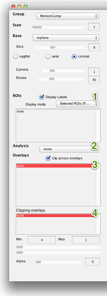
… your new mrLoadRet window should look different from what you are used to. The left-hand side of the GUI has been changed to allow you to work more easily with the multiple overlays and statistical maps that are created during the various GLM analyses.
3) Changes to the GUI
Most of the behaviour of the GUI elements has been preserved, but there are some important differences and additions. The order of the top left controllers for Group, Scan, Base, anatomical orientation, image gamma and image rotation have changed slightly but they behave in exactly the same way as in previous versions of the GUI. The main changes concern the ROI and Overlay controls:
- ROIs: the tickbox “Display Labels” controls the visibility of all the ROI labels; the pulldown menu allows you to select the way in which the ROIs (all, selected) are being displayed (voxels, perimeter). Finally, the listbox contains all the currently loaded ROIs and you can select one or more ROIs by left click and holding down the command (or shift) keys to modify your selection. This adds some very useful flexibility in keeping ROIs loaded but not displayed.
- Overlays: this listbox replaces the pulldown menu of the previous version of the GUI, allowing the selection of multiple overlays at once. The listbox shows all the overlays stored in an analysis but only the overlay(s) that are selected are displayed in false color over the base anatomy. Most of the time you'll only select one of these overlays. If you want to show two maps simultaneously, just set different color maps for each overlay (in Edit→Overlay→Edit Overlay). Another difference with the old GUI is that the min/max clipping values below do not apply to the overlays selected here (in #2), but to the overlays selected in the “Clipping Overlays” list box (see #3 just below).
- Clipping overlays: this is a list of the overlays that determine the visibility of the currently displayed overlay(s) (selected in #2). To change the threshold (clip value) associated with a given clipping overlay, select it in box #3 and change the values using the controls below. This will change the voxels visibility of the currently displayed overlay (selected in #2) according to the values of the current clipping overlay (selected in #3). In the previous version of the GUI, the list of clipping overlays would have included all the overlays loaded in the selected analysis (i.e. a voxel would be clipped out if it was clipped out of any of the overlay in the analysis). This is still the behaviour if 'Clip across overlays' is checked. However this behaviour is not suited for most uses of the GLM analysis results. In general, a given contrast map should be clipped according to either its own values or the values of its associated statistical map, or both. Therefore, when 'Clip across overlays' is not checked, the clipping overlays only consist of (1) the overlay itself and (2) its alpha overlay (if it is defined). For GLM analyses, the alpha overlay of a contrast map is set to its corresponding statistical map by default. Note that if several overlays are displayed simultaneously (in box #2), the list of overlays in box #3 is greyed out and it is not possible to change the clipping values. In order to change clipping values for multiple overlays, set all clipping values separately for each overlay to be displayed and then display them together.
See here for more details on controls for overlays.
4) Run a basic GLM analysis
When you start mrLoadRet in the folder for this data set, the results of a previously run analysis will be loaded up by default, to give you an idea of what the end point of this tutorial is. You can spend a bit of time familiarizing yourself with the new interface.
Once you are ready to move ahead: to start the GLM analysis afresh, select View→Remove Analysis from the mrLoadRet menu, which will remove the pre-computed results and maps.
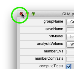
Clicking the menu item Analysis→GLM Analysis (v2) will bring up the first of a series of dialog windows that guides you through different settings and parameters you have to choose. Note that if you want to stop doing the analysis for any reason, you can cancel stepping through this process by closing the window (using the red window-close-icon in the top left corner of the dialog box). The “Cancel” button allows you to step back to the previous dialog window, if you eg realize a few steps in that you have entered the wrong value for one of the parameters.
GLM parameters
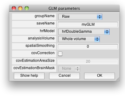
The first dialog window allows you to set up some general settings for the GLM analysis. You can specify what data that will be used for the GLM analysis (groupName), the name of the analysis/file to storing the results (saveName), etc…
- To make it easier to compare your results from running this tutorial with what you have downloaded, change the saveName to myGLM. This avoids a name clash with the pre-loaded analysis.
- To model the hemodynamic response, we will use a double-gamma model (hrfDoubleGamma). Other models include a simple boxcar (hrfBoxCar) and a more complex basis set model (hrfFslFlobs, which requires enabling the FSL plugin). You can also choose hrfDeconvolution to perform a deconvolution analysis.
- Perform the analysis over the Whole volume - if you have high-resolution data and very large matrix sizes, or if you want to increase power, you can choose to perform the GLM analysis on only a subset of the data to save time (and space). You can do this by first defining one or several ROIs and then choosing Loaded ROI(s) or Visible ROI(s) from this drop-down menu. This will spatially restrict your analysis to the union of all visible or all loaded ROIs. If you don't want to define an ROI, select Subset box and you will be prompted for coordinates of a subvolume in a later dialog.
- For this analysis, you can leave spatial smoothing parameter at 0 for no spatial smoothing. Increasing spatial smoothing will increase statistical power, but at the expense of spatial resolution. Unless resolution is critical for your research question, values equivalent to the FWHM of the hemodynamic response are recommended (~4mm at 3T and ~2mm at 7T, to be expressed in voxels).
- (noise) covariance correction is normally recommended but computationally expensive (could be several hours per scan unless you restrict your analysis to a small volume or have a lot of RAM). Leave the covCorrection box un-ticked - but read about corrections for noise covariance in the documentation.
For more information on all the parameters, as usual, select the 'Show Help' button or see the detailed GLM_v2 documentation . Press OK to proceed.
Model HRF parameters
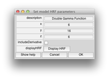
For a standard GLM analysis the HRF is assumed to have a standard/canonical shape that captures the temporally delayed and blurred haemodynamics. This dialog allows control over the parameters and lets you visualize the HRF shape.
The default parameters here are fine for the visual cortex (but might differ for other cortical areas). Click Display HRF to plot the model function. Close the plot window, then click OK to go to the next dialog.
Select scans
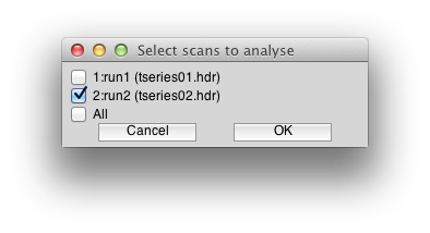
Determine which subset of scans in the selected Group are being analyzed. For starters, run the analysis on run 2. Select run 2 as shown and click OK to go to the next dialog.
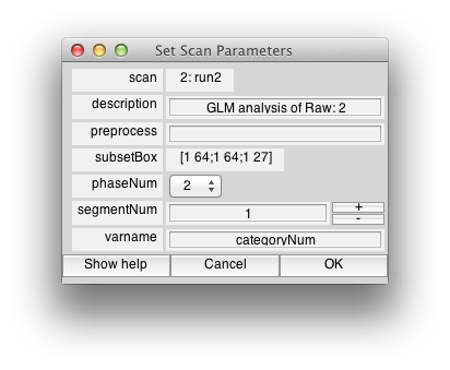
Select scan parameters
This dialog lets you specify how mrTools obtains the timing information about your experiments. For this tutorial data set, the timing is provided in MGL “stimfiles”. The stimulus code for this experiment implemented 3 “phases” of a task and a variable called “categoryNum” that specifies what objects were being displayed (phase #2, and segment #1 for each trial/block contains the relevant timing information). Set phaseNum, segmentNum, and varname according to the image and click OK to go move on.
Note that there are other ways to specify the timing of trials and blocks which may be useful to you if you use different stimulus setup (in particular the "mylog" format which is allows you to model the experimental design at a finer temporal resolution, see here).
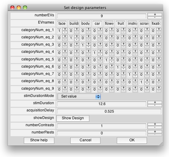
Select design parameters
In this dialog window you can further specify some details of how timing information is being used to create the design matrix for the GLM analysis.
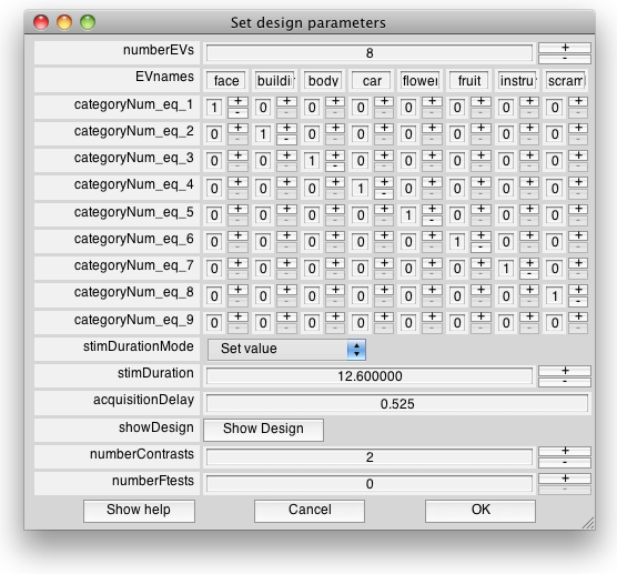
EVs, EVnames By default, one explanatory variable (EV) is set up for each unique value of the trial type variable you have provided (here, “categoryNum”). Change the EVnames to be useful & descriptive here and note that each EV corresponds to only one stimulus type (1's along the diagonal of the grid). Under some circumstances you might want to combine different trial types into a single EV at this stage, if e.g. different values of your variable correspond to identical stimulus conditions, and put several ones in a given EV column.
Note that the fixation periods in the beginning and end of the experiment (phases 1 and 3 in the MGL stimulus file) do not appear here because we have only selected phase 2 in the previous dialog. This is not an issue because these 'stimuli' correspond in fact to a baseline condition and do not need to be explicitly modeled.
For the same reason, we set the last stimulus type (fixation) to 0 here. One common pitfall in specifying the design matrix is to model all the conditions in your experiment, including the gray/rest periods explicitly. This is a bad idea, as it causes the design matrix to be rank-deficient and makes an important matrix in the calculation of the least-squares solution non-invertible.
stimDurationMode controls how the timing information is being used to construct the columns of the design matrix. For MGL stimfiles there are three options. (1) 'Event-related' for which each event is given the minimum possible duration (generally the duration of 1 TR). (2) 'Block' for which each event is assumed to run until the occurence of the next event/trial and (3) 'Set value' for which the stimDuration parameter is being used. Here, we use this third option. The appropriate value is 12.6 s.
acquisitionDelay is the time at which the fMRI data were actually acquired (on average for the stack). This is set to 1/2 the value of the TR, but for sparse imaging protocols this value might be different.
numberContrasts determines how many contrasts you will specify in a later dialog box. If you are not sure how many you want to do, err on the side of too many (add a couple extra for good measure) – it's easy to discard unwanted ones later. For now, set the value to 1.
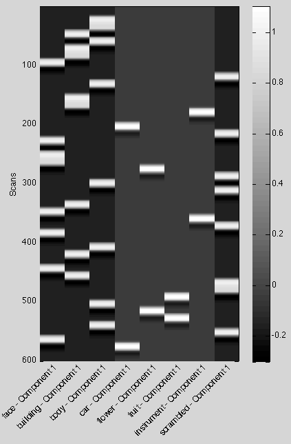
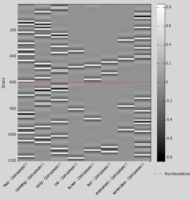
At this point, you can check that the timing information has been used in a way that you expected (and correctly): click on the Show Design button. This will pop up two extra windows showing the design matrix (grayscale image with multiple columns). Each column contains the prediction for one EV, time running from top to bottom. There is also a color image of the timing of the experimental design.
Statistics menu
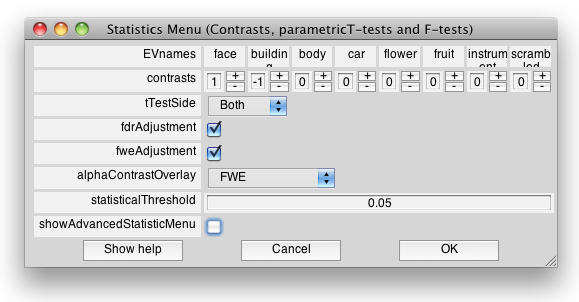
This dialog window is used to set the comparisons (contrasts) you want to test and specify the details of the statistical inference and thresholding that will be applied to the output overlays.
Each contrast is determined by a vector (row) that sets comparisons between the different explanatory variables (EVs, i.e. columns in the design matrix). For the purpose of this tutorial, we want to compare the responses to faces versus buildings – a comparison that is often made to isolate the fusiform face area (FFA) and other regions of ventral visual cortex that respond preferentially to images of faces.
To do this, we set up a contrast that highlights areas that respond more significantly in one condition than another, here e.g. “more to faces than to buildings. Bump up the value under 'face' to +1 and decrease that under 'building' to -1. This creates the contrast [+1 -1 0 0 0 0 0 0] which will compare the responses to categories 1 and 2 (the first two entries in the vector) and ignore the rest of the categories. Sometimes you'll want to look for responses to one stimulus type that are different from zero/baselines, rather than another condition – in this case you might have a contrast like [+1 0 0 0 0 0 0 0], to find areas that respond more significantly to faces than the baseline condition.
For details on how to set contrasts for GLM analyses, you might want to read eg. p 354ff in Huettel, Song & McCarthy and FSL overview of GLM analysis for details.
Because we don't have specific hypotheses about the direction of the effect (i.e. we want to reveal two sets of areas, ones that respond more vigorously to faces than buildings and other where the pattern is vice-versa), use a two-sided test and set tTestSide to Both.
The next choice you have to make is whether you want to look maps that have been adjusted for false-discovery rate (FDR) or family-wise error rate (FWE). If you select both, you have a choice of looking at the data under both schemes later. The statistical maps will be thresholded, but to aid visualization, their voxel-wise transparency will also be adjusted according to a map of your choosing. For, now set this alphaContrastOverlay to FWE and leave the statisticalThreshold at the default 0.05 (corrected). Note that output maps are not hard-thresholded, meaning that it is possible to increase/decrease the threshold after the analysis has run.
Selecting the showAdvancedStatisticsMenu will interpose another dialog window with additional options for advanced use (some of which are experimental or computationally expensive or both, see the detailed documentation and a full description of the advanced statistical options). For now, leave this box unticked and click OK to move the analysis along. At this point, the GLM analysis will actually run and it may take a minute or so to complete, depending on your hardware and memory settings.
Quick aside; F-tests
If you want to test the overall significance of a collection of contrasts (without making any assumptions about their relative weights), then F-tests are a way to achieve this. If you select to calculate F-tests in the design menu, then the Statistics dialog box will allow you to specify a “restriction matrix”. Details on this are in the documentation and in Burock & Dale (2000). Note that the fContrasts matrix that you specify need to be of full rank - if not, you should be warned that the fContrast is invalid.
5) Visualizing and interpreting the results
Once the calculation is complete, the analysis will be automatically saved. If you've not changed the name of the analysis, you will be asked whether you want to overwrite the pre-loaded analysis, rename the new analysis or merge the two analyses. We suggest you save your effort as a new analysis (e.g. myGLM) and keep the one that you downloaded for now so you can compare and check that you obtained the same maps. You may have to load the file we have provided again, but as long as the saveNames are different, you will be able to have any number of analyses loaded at the same time.
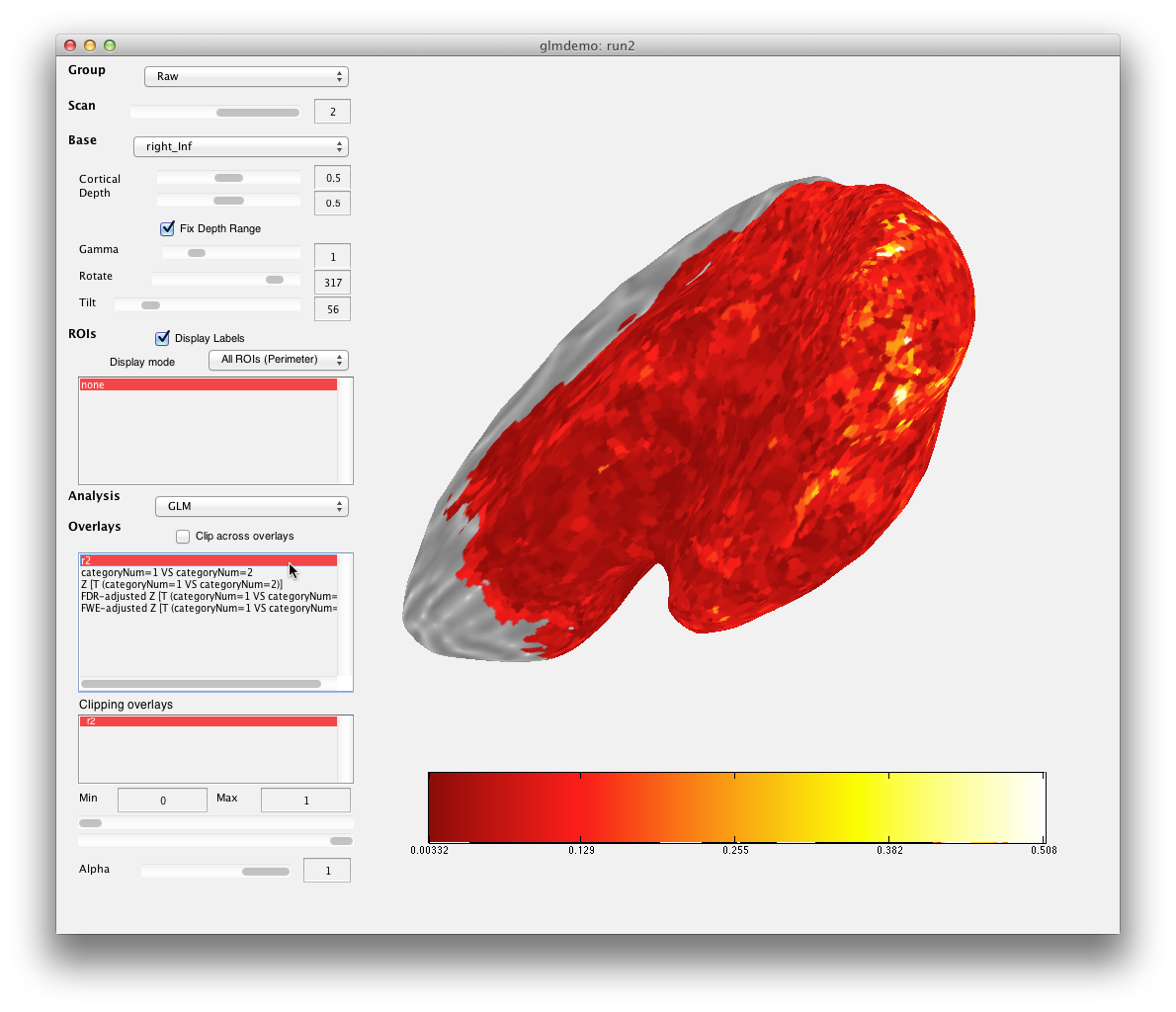
The result of the GLM analysis are 5 overlays:
- r2 - proportion of variance explained by the model
- categoryNum=1 VS categoryNum=2 - the contrast values
- P [T(categoryNum=1 VS categoryNum=2)] - uncorrected statistical significance of the contrast
- FDR-adjusted P [T(categoryNum=1 VS categoryNum=2)] - FDR adjusted significance
- FWE-adjusted P [T(categoryNum=1 VS categoryNum=2)] - FWE adjusted significance
Look at each of these maps in turn (make sure interpMethod is set to Nearest in Edit→Preferences so that your results appear identical to the screen captures shown here).
The r2 map shows how well the model fit the data overall (proportion of variance accounted for at each voxel). You may have seen these kinds of maps in the eventRelated analysis and the previous implementation of the GLM tools.
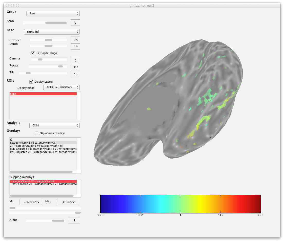
The second map shows you the results of the face-vs-building contrast that was calculated:
- each voxel that is rendered in color survived the thresholding we applied. If you select the second overlay (FDR corrected) in the “clipping overlays” listbox, you will see that the threshold is set to p=0.05. Try increasing this threshold and note that this adds a few voxels to the display
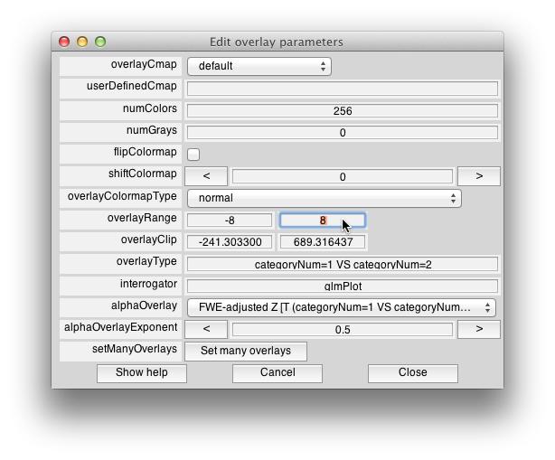
- the colors are given by the contrast values and how they are mapped to the colormap - you can change this by changing the overlay range in Edit→Overlay→Edit Overlay from [-36 36] to a tighter range e.g. [-8 8].
In this dialog, you can also select a different statistical map to mask the contrast overlay. Try selecting a different alphaOverlay (e.g. uncorrected or FDR-corrected) and see the effect on the displayed contrast map. Close the dialog when you're done.
Maps of significance are rendered as P maps by default (depicted here without thresholding). You might find that looking at Z maps offers a better color dynamic range. To display Z values, you need to re-compute the analysis. You can easily go back to this via Analysis→Edit Params & Recompute without having to enter all parameters of your analysis again. In the last dialog, check showAdvancedStatisticMenu and press OK. You will then be presented with an additional dialog. Select Z value for the testOutput parameter, press OK and select Overwrite when prompted.
Note that larger Z values correspond to more significant results and that the p=0.05 threshold has been converted to a Z=1.644853. Note also that Z values cannot increase above 8.209536, which corresponds to a minimum p value of 10e-16.If you prefer getting Z-values or -log10(P) rather than P values by default (i.e. without having to go into the advanced options), you can set the mrPreference statisticalTestOutput to the appropriate value:
>> mrSetPref('statisticalTestOutput','Z value');
6) Visualizing multiple contrasts on a single map
Next we will perform a different analysis to compare the spatial distribution of voxels that prefer a) faces over objects and b) bodies over objects. To increase our statistical power, we will run the analysis on both runs 1 and 2.
Concatenation and temporal filtering
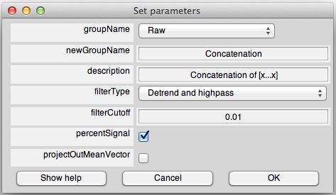
First you need to concatenate the two runs in group Raw, select Analysis→Concatenate Time Series.
Click OK to accept the default options which include temporal detrending and high pass filtering at 0.01 Hz.
Then select runs 1 and 2 and click OK. Once the calculation has completed, use the GUI Group selector to switch to group Concatenation. As usual, verify the quality of the concatenated time series by using the interrogator to plot some voxel time courses, and the Plots - Display EPI images tool to compare EPI images around the border of the original scans.
Calculating the contrasts
To compute the new contrasts, you will have to re-run the GLM analysis. It is possible to retrieve the parameters from our first analysis and apply them to the new concatenated scan: First switch back to group Raw and select Analysis→Edit Params & Recompute. Then change the group name to 'Concatenation'. The other parameters should be set to the same values as previously. Click OK here and in the following dialog.
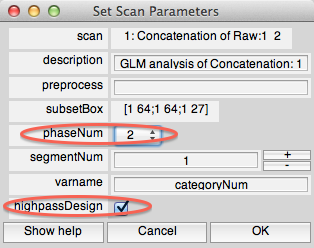
In the 'Set Scan Parameters' dialog box, set phaseNumnote to 2 and note that highPassDesign is checked by default, meaning that the same temporal filter that was applied to the time series during concatenation will also be applied to the GLM design matrix.
Next, you come to the “Set design parameters” dialog. There, reset stimDurationMode to Set value and stimDuration to 12.6.
Then click the Show Design button to confirm that the stimulus files link appropriately to the concatenated file. The design should look like this:
Note the dashed lines that separate the two runs in both figures. Close these two figures and go back to the Set design parameters dialog. Set numberContrasts to 2 and click OK.
Now we come to the StatisticsMenu (Contrasts, parametricT-tests and F-tests). With the first contrast, we will look for voxels that preferred faces over “mixed objects” (cars, flowers, fruit and musical instruments). Such (balanced) contrast is defined with coefficients [1 0 0 -0.25 -0.25 -0.25 -0.25 0]. With the second contrast, we look for voxels that prefer human bodies over mixed objects [0 0 1 -0.25 -0.25 -0.25 -0.25 0]. Keep the other parameters as before except for tTestSide: we will now use a right one-tailed T-test because we are only interested in voxels whose response is stronger for faces/bodies than objects (also uncheck advancedStatisticsMenu if you have checked it previously).
Click OK to start the calculation, which should take longer than previously. Note that a warning is issued that the two contrasts are not orthogonal.
Editing and displaying the contrast overlays
You may want to explore the results as described in Looking_at_the_results. Then, we will modify the overlays for a simultaneous display of face and body preferring areas. To compare your results to the screen captures shown here, rotate the surface to expose the lateral part of the occipital lobe.
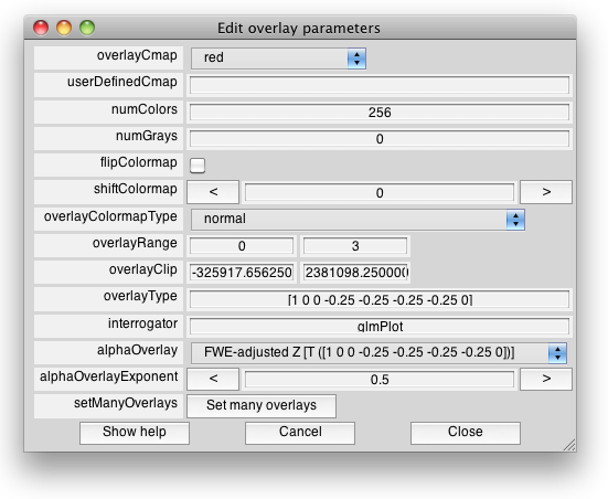
First, in the Overlays list in the main GUI, select the faces > objects contrast ([1 0 0 -0.25 -0.25 -0.25 -0.25 0 ]). Then go to Edit→Overlay→Edit Overlay.
- Change overlayCmap to “red” near the bottom of the list
- Change overlayRange to 0…3 to compress the color scale to a relevant range
Leaving the Edit Overlay dialog open, now select the bodies > objects contrast ([0 0 1 -0.25 -0.25 -0.25 -0.25 0 0]) in the Overlays list. This should load the appropriate overlay parameters in the Edit dialog. Make the same changes as above, but pick a blue color map. Click Close to close the dialog.
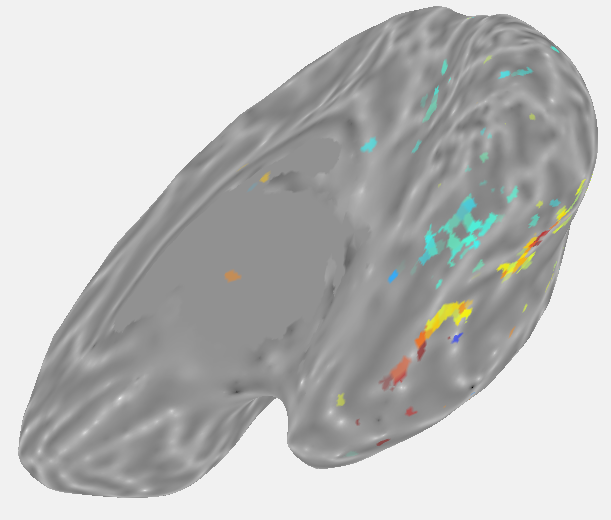
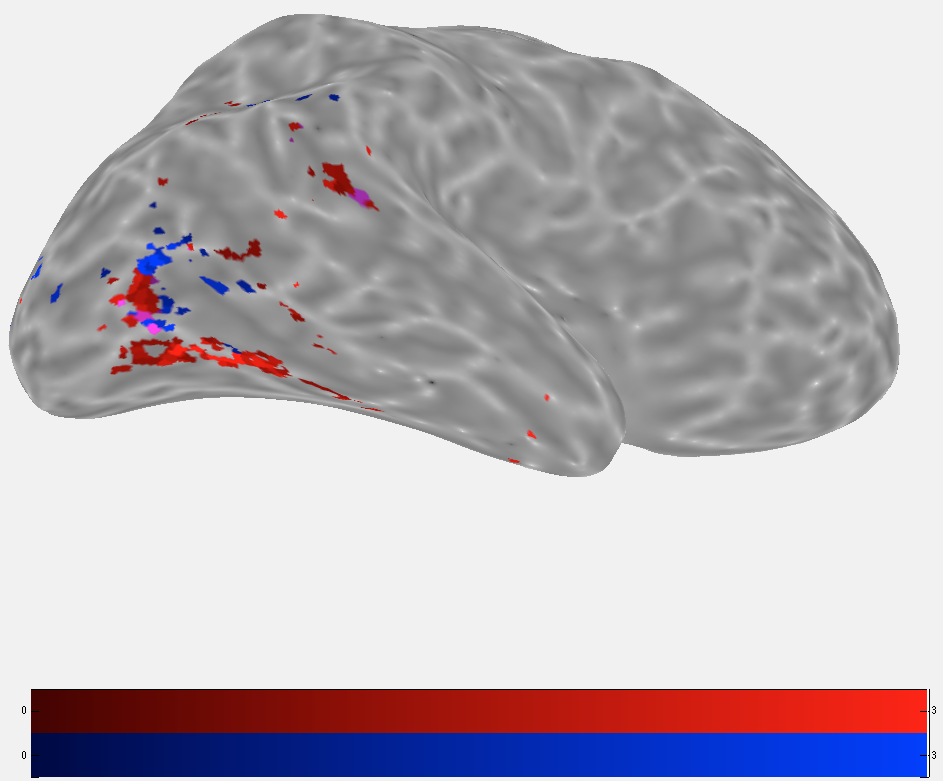
Now we are ready to display face and body areas simultaneously. Use Command (or Control) - LeftClick to select both contrasts ([1 0 0 …] and [0 0 1 …]) in the Overlays list. You should see the following plot, where red indicates face preferring areas, blue body preferring areas, and tones of purple/pink mark voxels that respond to both categories.
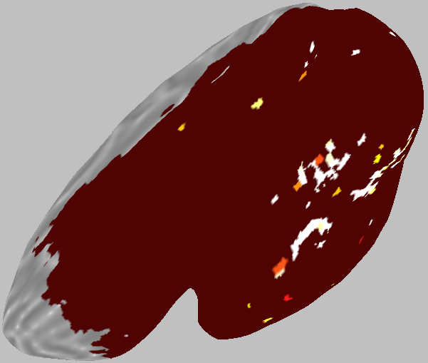
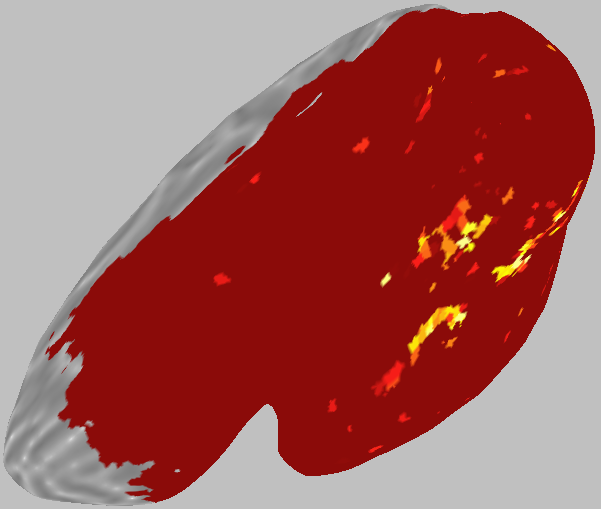
Note that we are plotting contrast values, but they are thresholded by FWE-adjusted P values. To adjust the statistical threshold, click on one of the contrasts in the Overlays list in the main GUI. Then go to the Clipping overlays list and select FWE adjusted P. Corresponding to the default values we accepted when setting the parameters for GLM calculation, the range is from 0 to 0.05, i.e., p < 0.05. You can try a more conservative threshold by setting the max to 0.01 or 0.001. You need to adjust this setting separately for the face and body contrasts. Then use Command-click again to display them simultaneously.
GLM plots: plotting estimated beta values for all categories and contrasts
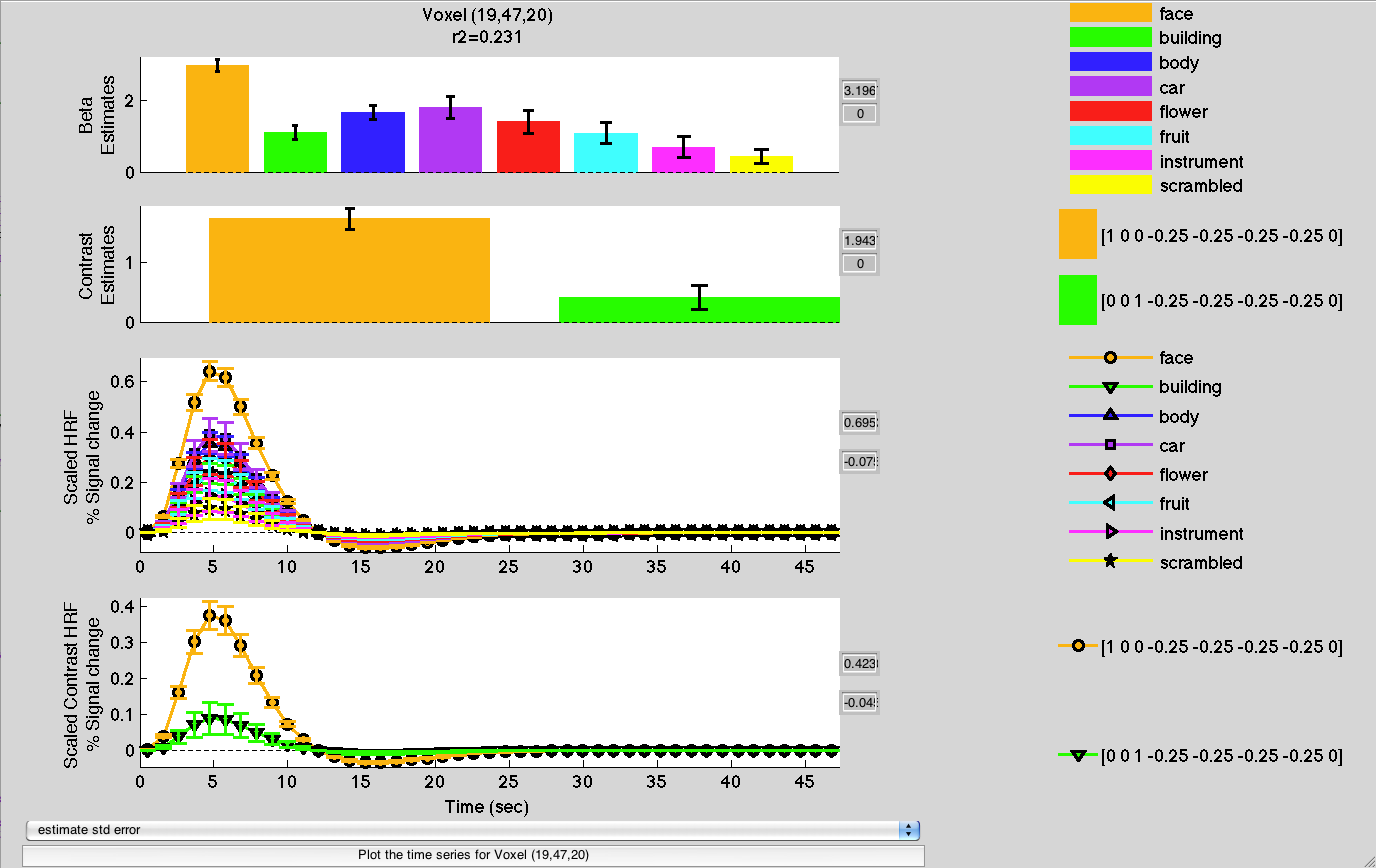
To get an idea of the overall response profile of a given voxel, we can use the Interrogator. Go to Plots→Interrogate Overlay. Then Click on a red face voxel, and you should get something like shown below. The top row shows the EV parameter estimates for each category, which are about twice as high for faces than for other categories. The second row shows the contrast values: the first contrast (face vs object) has a large value, but the second one (body vs object) has a low value because for this voxel the GLM beta estimates for bodies and objects were similar. The two other rows show the model HDRs, for each EV and contrast respectively, scaled by the parameter/contrast estimates.
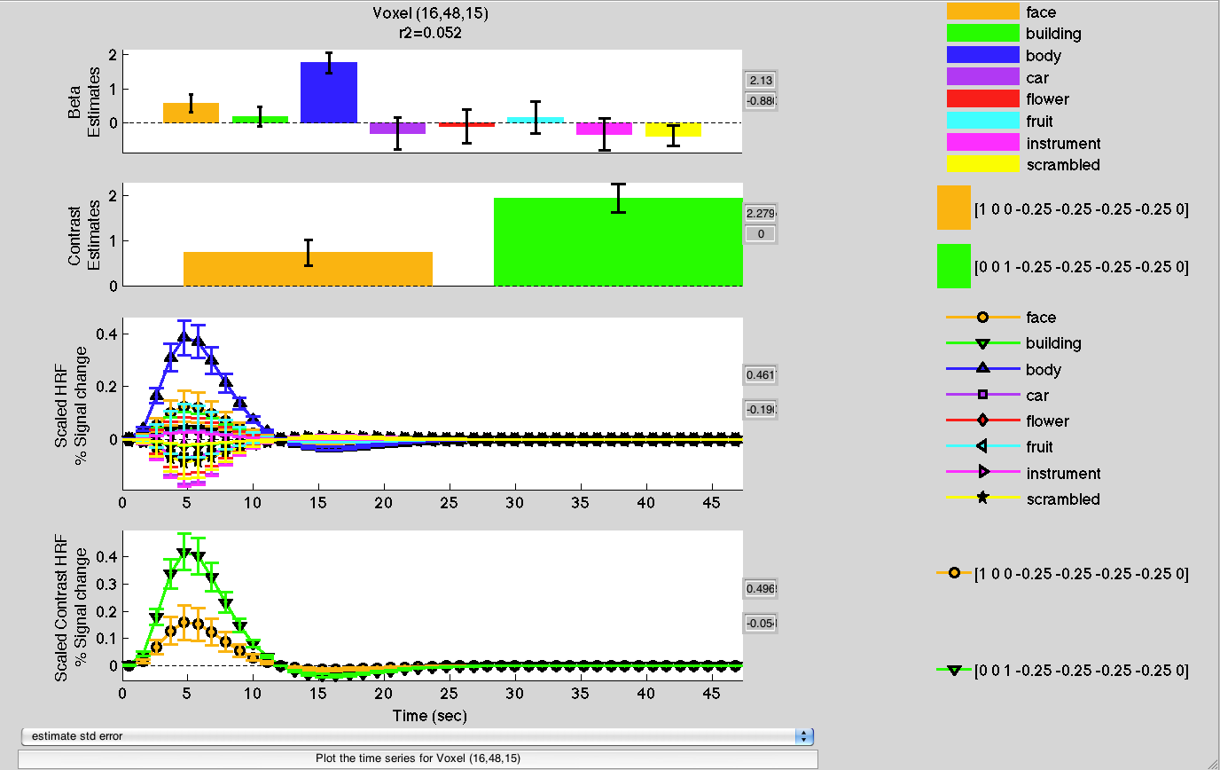
For a body-preferring voxel, we observe a very different pattern:
Explore overlays, statistical maps, etc.
Note on overlays, color maps, etc.
- each overlay is associated with one or more clipping overlays
- contrast overlays usually have an associated P/Z alpha overlay, which determines transparency, unless you selected 'none' in the alphaContrastOverlay field of the Statistics menu. If you want to remove this (or change the map that provides alpha transparency), you can edit this in the settings for the selected overlay: Edit→Overlay→Edit Overlay
- you can select + display multiple overlays at the same time; this feature is useful if you have e.g. two contrasts highlighting two areas, say one responding more to motion stimuli, others more to images of objects. Change the colormap associated with one of the maps, shift-select both overlays and mrLoadRet will display the two maps with their associates colormaps (see section on “Visualizing multiple contrasts” above).
- if there is more than one clipping overlay, you can further refine the display by selecting one and adjusting the Min/Max values. For example, the display of a beta map can be thresholded by itself, allowing you display only voxels with positive beta values. (see section on “Visualizing multiple contrasts” above). This is in addition to the Z (or p) maps that you would normally use to modify the significance thresholds.
7) Advanced features
For more complicated experimental designs or advanced statistics, look at the detailed explanation of GLM_v2 which covers more technical details of the implementation, including:
ds, tt and jb - June 18th 2013

