This tutorial will show you how to import a surface segmentation into mrLoadRet so that you can view your data on a surface. It will also show you how to make a flat map from that surface.

1. Download tutorial data
2. Create a curvature file
3. Load event-related analysis to view on inplane anatomy
4. Import surface
5. Create a flatmap
6. Finding voxels in different anatomies
7. Inflated surface

You can download the tutorial files from:

http://www.cns.nyu.edu/heegerlab/content/software/mrLoadRet/surfTutorial.tar.gz

The files are provided as a tar/zip file. In Mac OS X you should be able to just click to open the files in the Finder. Otherwise, you can go to a terminal and do:

gunzip surfTutorial.tar.gz
tar xvf surfTutorial.tar

We assume that you have mrTools running on your system. This is a paired down version of the same dataset as the Event-related Tutorial. To make it easier to download it does not include all the data files, so you cannot rerun analyses on this example. The data has already been motion corrected, aligned to the 3D volume using mrAlign, concatenated and the eventRelated analysis has been run.

To view your data on a surface, mrLoadRet needs a segmentation. A segmentation consists of two surfaces, one that tells where the outer (pial) layer of the gray matter is and one that tells where the inner layer is (between the white matter and the gray matter). These files can be created by any segmentation tool as long as they are in .off format. We typically use FreeSurfer (see here for how to import) to generate segmentations. Jonas Larsson's SurfRelax and Caret (though Caret only produces a mid-cortex surface and not the outer and inner surface as we like to use. see here to import) can also be used.

Once you have a segmentation, mrLoadRet also needs a file which tells it how to color the surface. We use the curvature to color the surface. In this tutorial we have provided an outer and inner surface for the left cortex, but no curvature file. You thus need to create the curvature file:

First cd into the Segmentation folder:

cd Segmentation

You should see the following files:

>> ls
leftOuter.off     volume.img
leftInner.off     volume.hdr

Now generate the curvature from the inner surface

m = calcCurvature('leftInner','leftOuter');

And then save it in vff format:

saveVFF('leftCurvature.vff',m)

First, we will start up mrLoadRet

cd surfTutorial
mrLoadRet

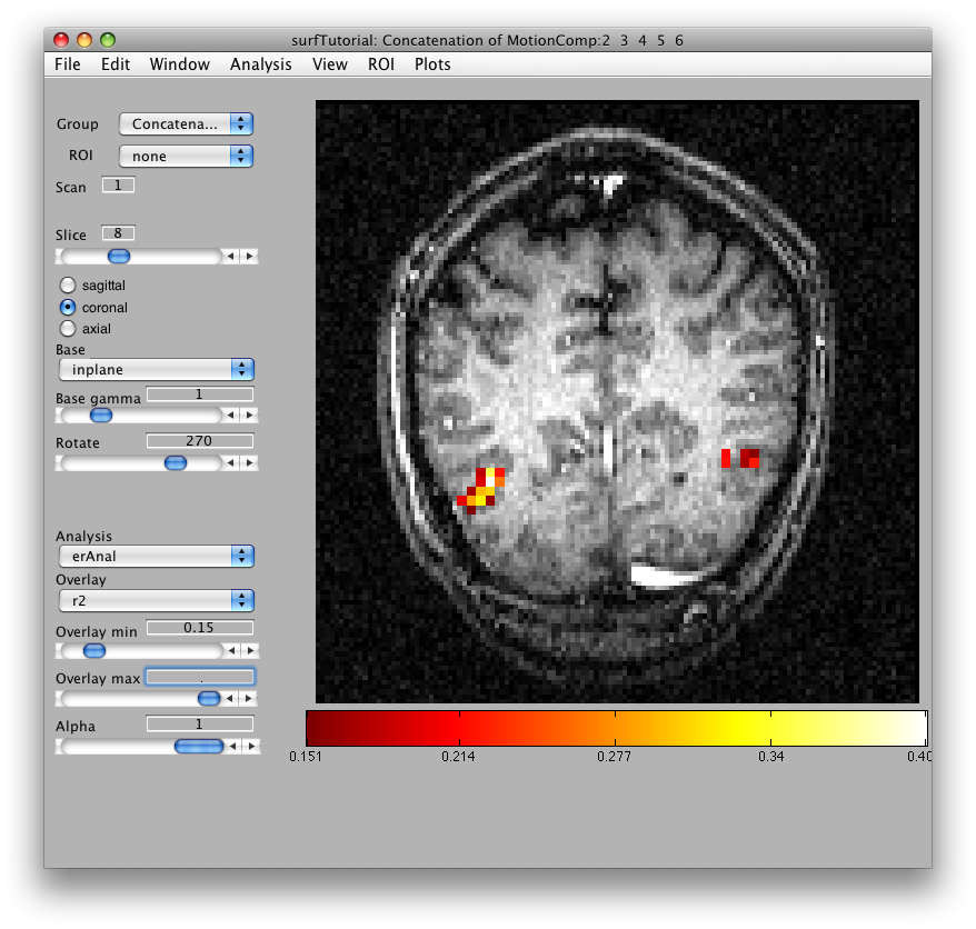
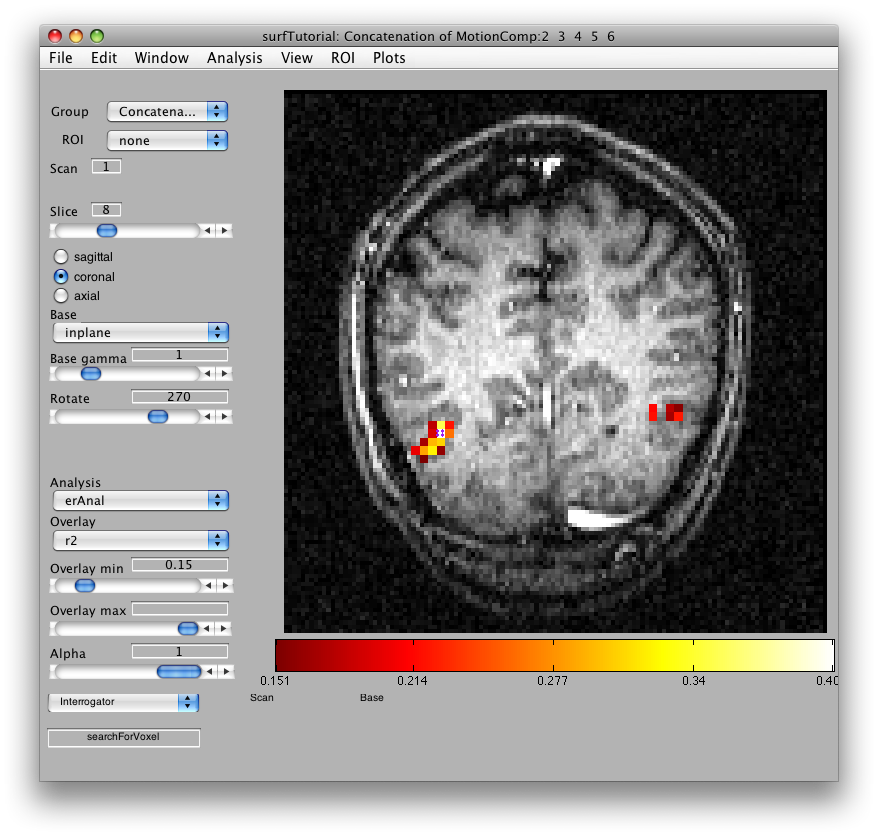
Then we will load the already computed event-related analysis and view it on the 2D inplane anatomy. Make sure you are on the Concatenation group and then from File/Analysis/Load, load erAnal/erAnal.mat. Set the Overlay Min to 0.15, the Slice to 8, and you should see (you might need to go to slice 15 and set Rotate to 90):

Now, we are ready to import the surface. Go to File/Base Anatomy/Import Surface, and find the outer surface file in the segmentation directory (i.e. Segmentation/leftOuter.off) and click Open.

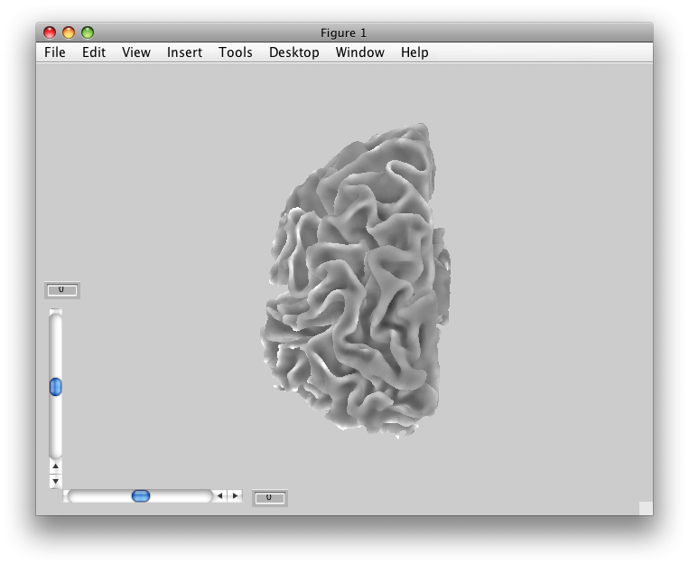
You should now see a view of the surface like this:

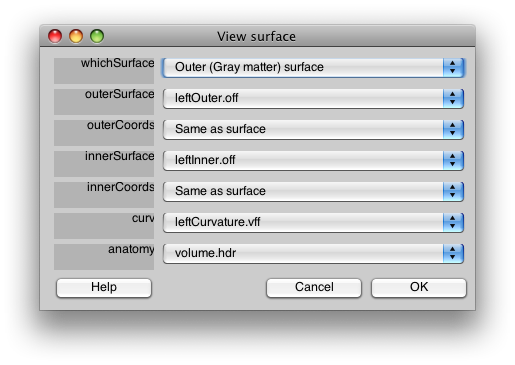
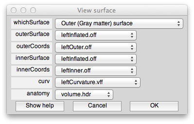
With a set of controls that look like:

This dialog should have the correct settings to load your surface already, but it allows you to make changes and selections. The surfaces appear four times in the dialog. This is because there is a distinction between a display surface and a coords surface. The display surface is the surface that will be actually drawn. The coords surface specifies where the data for the displayed surface comes from. In our case these are one and the same, but if you were displaying on an inflated surface, for example, you would want the display surface to be the inflated surface and the coords surface to be the gray matter surface. The outer and inner surfaces are what will be displayed when the cortical depth slider (more later on this) is set to 1 and 0, respectively.

The other files you see here are the curvature file which is simply how to color the surface. The anatomy file is the 3D volume anatomy from which these surfaces were segmented. It is important to have this file since it contains the right transformation matrix that is needed to transform data on to the surface to be displayed.

At the top of the dialog, you will see a field called “whichSurface” this chooses which surface that is currently being displayed. This is there so that you can inspect all the surfaces to make sure you have chosen the right one. For example, set it to Inner (White matter) surface, and you should see:

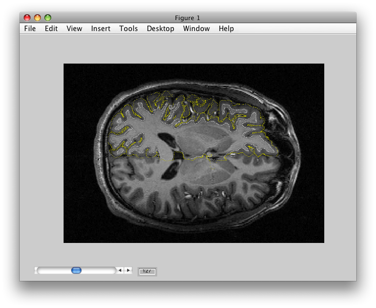
If you set whichSurface to 3D Anatomy, you should see this:

The 3D Anatomy is particularly important to inspect. The yellow line shows you where the outer coords are being taken from. It should follow the outer surface of the gray matter. The data that will be displayed will always come from the location of where the yellow line is, if you set the cortical depth to 1. There is also a white line. This should follow the inner surface of the gray matter. It is where data will be interpolated from when you set the cortical depth to 0. When you set the cortical depth to an intermediate value (e.g. 0.7) it will interpolate the data from the appropriate depth between the inner and outer surface.

Again, it is a very good idea to look at this view carefully to understand how good your segmentation was.

When you are done, click OK.

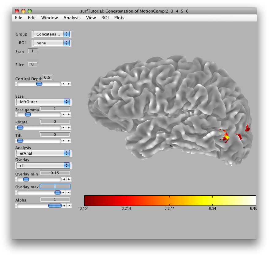
In a moment, you should see in the main viewer, something like this:

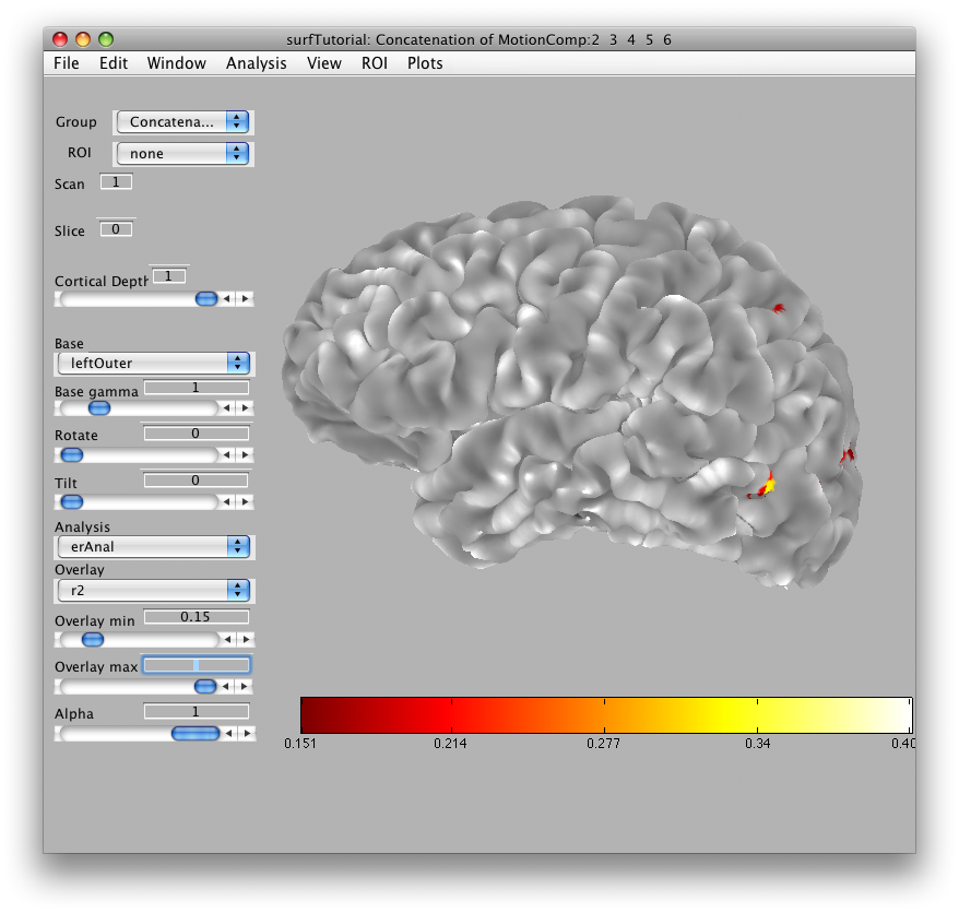
You can use the rotate and tilt sliders to rotate and tilt the surface. You can also change the cortical depth that is being displayed. When you set the cortical depth to 1, you will see the outer surface:

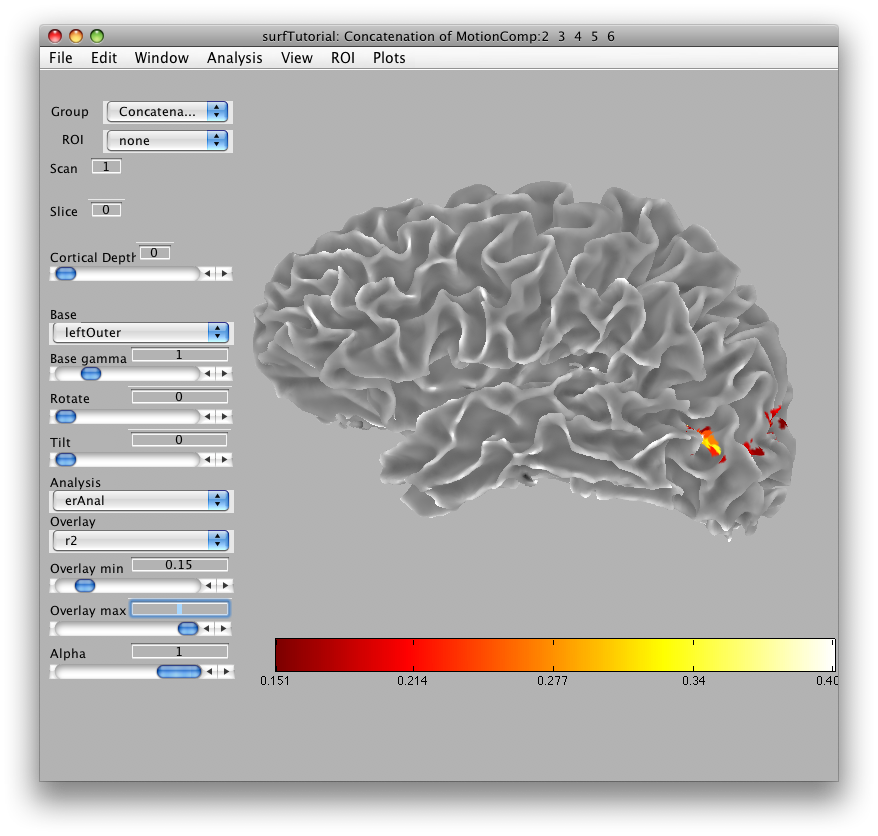
When you set the cortical depth to 0, you should see the inner surface:

Note that if you ever want to go back to look at the files that created the surface, you can always go to Plots/Surface Viewer.

Now that you have imported the surface, you may want to save it in a format the MLR can read directly. First, you may want to change its name, which you can do by going to Edit/Base Anatomy/Edit Base Anatomy and then setting the baseAnatomy. Next, go and save by going to File/Base Anatomy/Save. This will save a file that can be directly read back into MLR without importing into the Anatomy directory. If you wanted to save to a different directory (for instance the volumeDirectory repository which you should set in Edit/Preferences volumeDirectory), then click on File/Base Anatomy/Save As… and it will bring up file save dialog which opens up to the Edit/Preferences volumeDirectory.

Now that you have the surface loaded, it is easy to make a flat patch of any location you want.

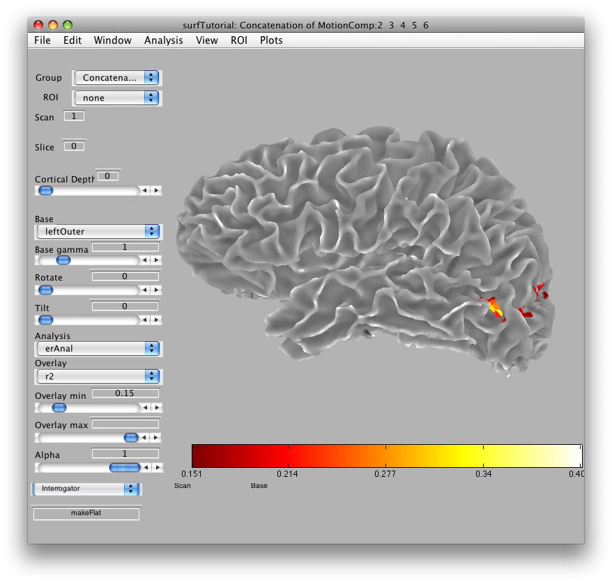
Go to Plots/Interrogator Overlay and turn the interrogator on (by clicking). In the bottom left of the viewer, select “makeFlat” as the interrogator from the drop down list box, so that makeFlat should now appear in the text box at the bottom left of the viewer:

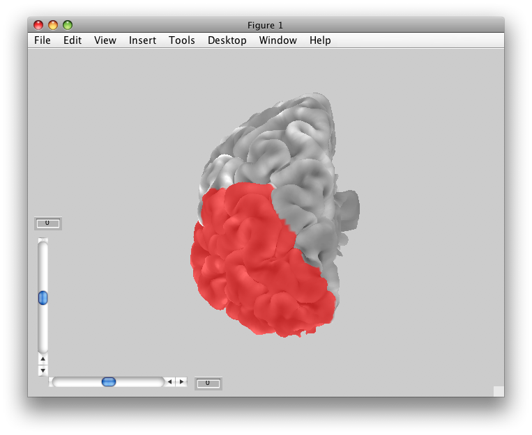
You can now click on any portion of the surface that you want to flatten. For instance, the patch of brightly colored voxels that you see in the mid-occipital cortex is MT. Click on that, and you should see a preview of the flat patch to be made that looks like:

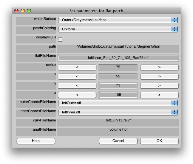
And you will get a parameter dialog that looks like:

Like last time, you can look at the various surfaces, by changing “whichSurface”. You can also change the way the patch is colored, for example, try “Current Overlay with Patch” in “patchColoring” and then you should be able to tell if the patch you are making covers the whole area of activated cortex that you are interested in. You can also change the radius of the patch to make it bigger or smaller.

The only parameter we need to change though is the name. Change the flatFileName “leftInner_Flat_52_71_105_Rad75.off” to “leftMT” and click OK>

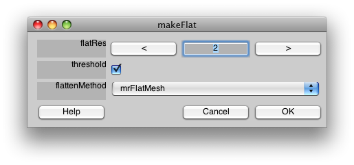
You should then see the following dialog:

The flatRes is the “resolution” of the flat patch. The flat patch will be converted from a true surface into a 2D image, and the resolution refers to how high a resolution you want to represent that flat image with. 2 is usually a good number, but if the resulting flat patch looks pixellated, you may try a higher resolution. The threshold check box, will make it so that the curvature is threshold, making a two color flat patch. If you want to have the smooth curvature displayed instead, turn off the threshold.

flattenMethod selects which system to use to flatten the patch. We typically use mrFlatMesh, which is a modified version of the code that came from the Stanford Vista package developed by Brian Wandell's lab. If you are using Jonas Larsson's SurfRelax tools and have those properly installed, you can choose SurfRelax and try that.

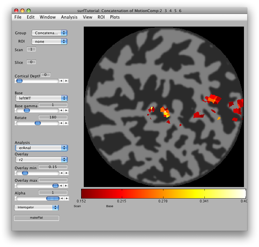
Select mrFlatMesh as the flattenMethod and click OK. After a few minutes, you should see:

Note that you may need to rotate the patch to get it in the same orientation. In general, you should try to orient your patches such that dorsal is up and ventral is down - the next section which shows you how to search for voxels is useful for this, particular in the “continuous mode” described below which will show you which part of the patch is at the top and bottom of the brain.

You are now done making your first flat patch.

If you want to go back to the view of the flat patch on the surface, you can select Plots/Flat Viewer. This is a useful thing to do, since you can also see how the patch is oriented and see how much distortion is in the patch.

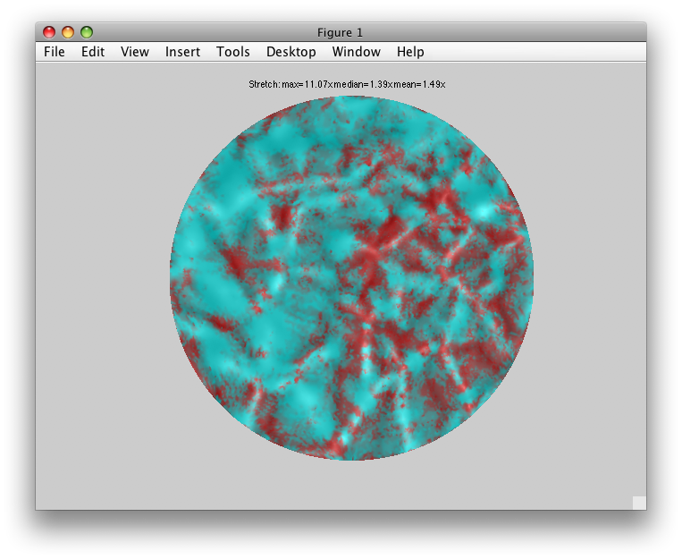
For example, from the Flat Viewer, select “whichSurface” to be “Patch” and “patchColoring” to be “Stretched areas in Red”. You should see something like:

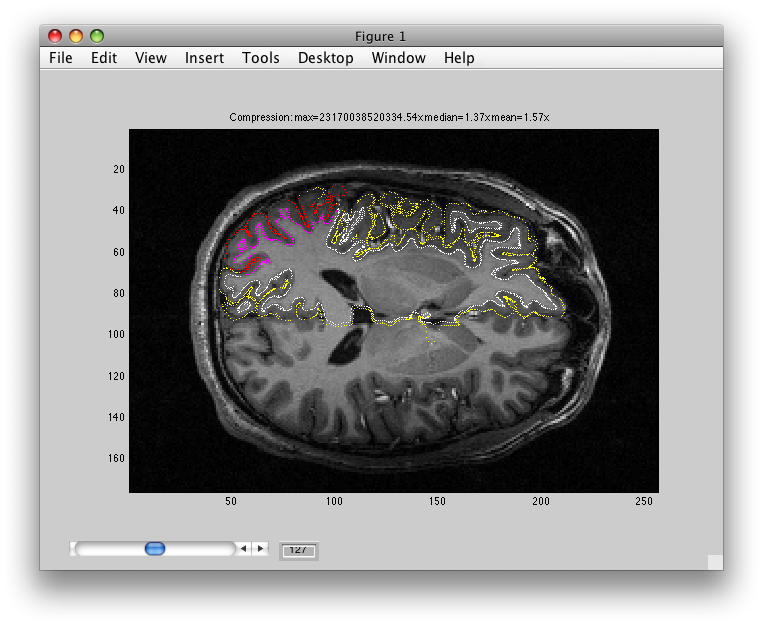
You may also want to see where your patch coordinates are coming from on the volume anatomy. Choose “patchColoring” to be “Uniform” and “whichSurface” to be “3D Anatomy” and you should see:

The yellow and white are the same as before (your outer and inner surface boundaries). But, the Red and Pink parts are the outer and inner coords for your flat patch.

You can click OK to get out of the Flat Viewer.

You may also now want to change the baseName and save the flat patch to a native MLR format (nifti pair with associated matlab file) by following the directions above at the end of the section on Importing a surface. Note that when you save it will save the default rotation and other parameters so that the next time you load it the flat patch will be oriented correctly.

Some times it can be very confusing looking at a flat patch and deciding where a particular voxel of data came from. One way to figure that out is to use the “searchForVoxel” interrogator.

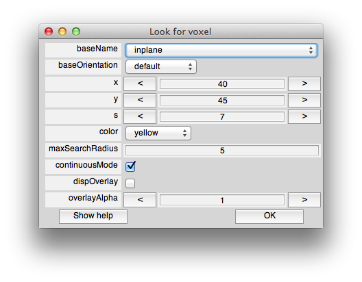
You should still have the interrogator on (Plots/Interrogator). Now select searchForVoxel in the drop down list box at the bottom left of the viewer, and “searchForVoxel” should now appear in the iterrogator text box. Now if you click on one of the activated voxels in the center of the patch, you should get a dialog like this:

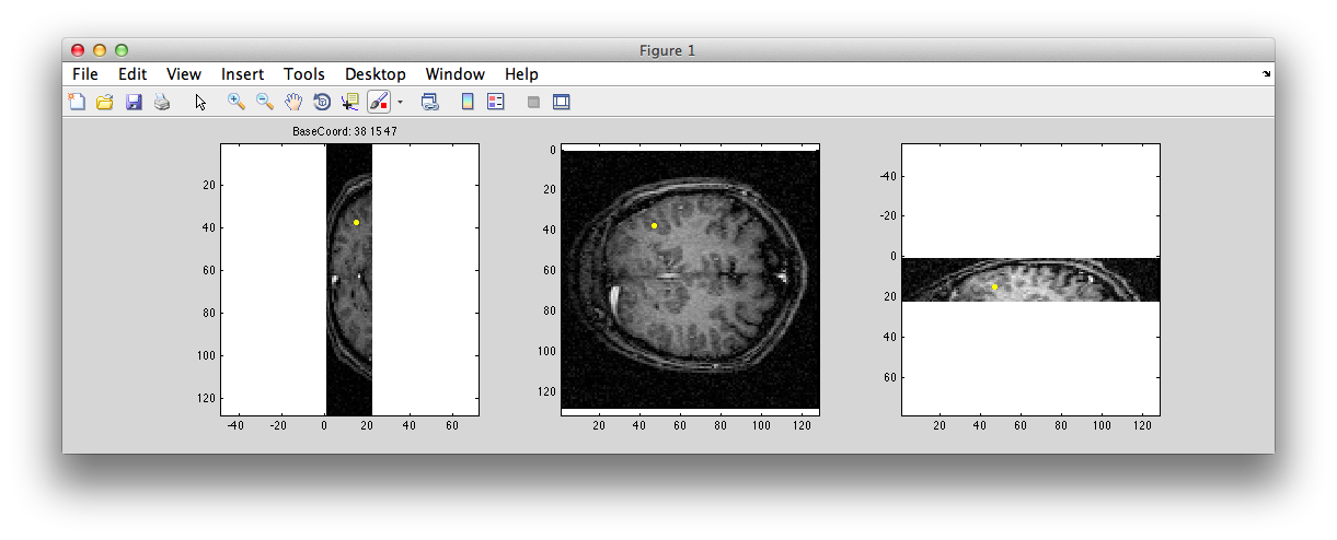
Assuming continuousMode is checked, then as you move your mouse over the flat patch in the main viewer, you should see a little yellow dot move around in another figure window that pops up like this:

The little yellow dot should run around in there as you move the mouse over the flat in the main viewer indicating its location in the inplane anatomy. This can be very helpful in determining where points came from in the flat. If you have a full 3D canonical available (not in this tutorial), you could switch to that anatomy in the dialog box shown above and it will show you in that anatomy.

The following feature has been a bit superseded by the continuous mode (you can avoid doing it by closing the dialog box by clicking on the red x button at the top left), but if you choose “inplane” for the baseName, and set the color to purple (so that it will be easier to see) and click OK, then it should switch you in the main viewer to the inplane anatomy and it should look like this:

Notice the four purple little points that are drawn over one of the voxels on the left side. This is where the voxel you clicked on in the surface came from.

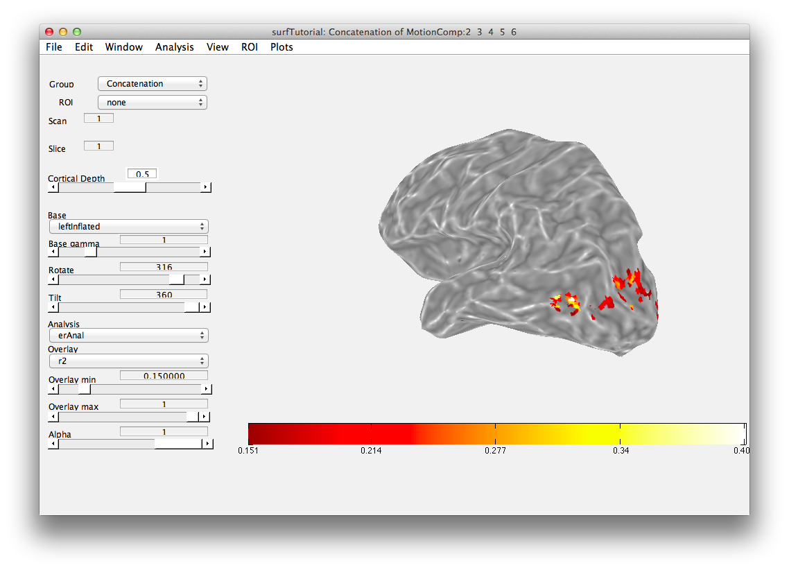
Often it is convenient to make an inflated surface to display your data on. This is easy to do by using the inflated surface that FreeSurfer creates. Go to File/Base Anatomy/Import Surface, find leftInflated.off from the Segmentation directory. Now you just have to set the outer and inner coords appropriately (obviously you don't want to use the coordinates of the inflated surface since those are in the wrong place and should be used for visualization only). Your dialog should look like this:

When you click ok, you should get a surface in the viewer that looks like this:

-jg.