Table of Contents
Layer fMRI and VASO Tutorial
This tutorial explains how to do layer fMRI analysis using mrTools. Much of this pipeline was developed by Renzo Huber and is described on his blog, though several steps have been adapted to mrTools. A number of software packages are required in addition to mrTools, including FSLeyes, ANTs, itk-SNAP, and LAYNII, and Eli's layer analysis MLR functions github repository.
Overview
- Preprocess the data
- Align the data with standard mrTools methods
- Draw inner and outer surfaces with fsleyes.app
- Grow layers with LAYNII
- Create mrTools ROIs from layer mask
- Plot layer profiles
1. Preprocess the data
1.1 Motion correction for VASO data
I have been using standard mrTools motionComp, with the tSmooth option set to 2. This flag averages n frames before and after the frame that is being registered. I think this helps with VASO registration for the following reason. The alternating images of nulled and not-nulled contrast have slightly different spatial profiles of image intensity. If you register each frame independently to a base image (without averaging), a slightly different transform is computed for nulled and not-nulled images. So, if you don't set the tSmooth flag, the resulting motionComp transforms have an alternating sawtooth pattern - that is bad. Setting tSmooth seems to fix this. I also recommend using 'cubic' interpolation, which blurs the data less than the standard 'linear' option. Renzo has an entire blog post on motion correction for VASO.
1.2 Computing VASO contrast from not-nulled (BOLD) and blood-nulled images
The time series in a VASO scan consists of alternating images of BOLD and blood-nulled contrast. VASO is computed by dividing the blood-nulled images by the BOLD images. The result is a measure of cerebral blood volume, and is a negative contrast (more negative means larger response). The matlab function 'computeVaso' takes each scan in the MotionComp group in mrLoadRet, separates the BOLD and nulled images, temporally upsamples them to be on the same temporal grid, divides one by the other, creates two new MLR groups ('Bold' and 'Vaso') and saves out the appropriate tSeries files to each group.
>> computeVaso
1.3 computing T1 from VASO time series
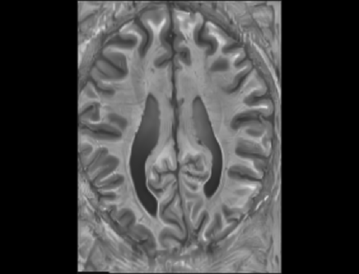
We want to define layers on an anatomical image that has the same spatial distortions as our functional images. To do this, we estimate a T1 image from the VASO time series. Once motionComp has been run, just run this matlab function, which will create vasoAnat and vasoAnatUpsampled in the Anatomy directory.
>> makeVasoAnat
1.4 registering, averaging, and denoising MP2RAGE anatomicals
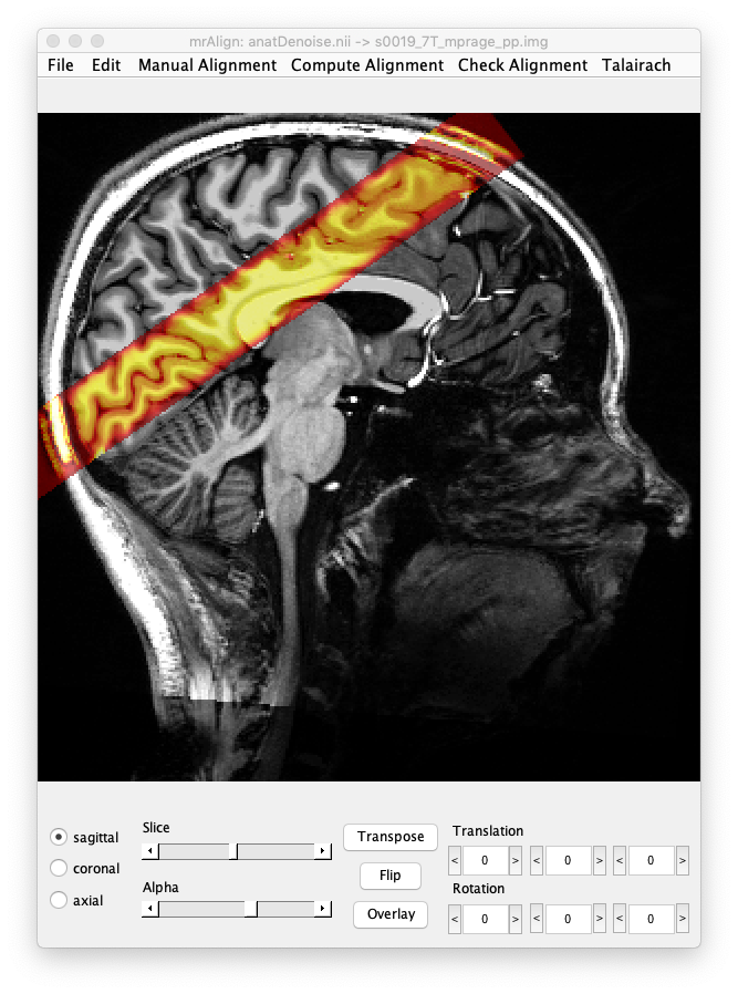
We typically collect multiple “in plane” MP2RAGE T1-weighted anatomical scans in the same session as the VASO data. These are typically 0.5×0.5×0.5 mm, and have the same slice angle and field of view as the VASO scans. Even though we are going to use the vasoAnat to draw the layer boundaries, this MP2RAGE scan is useful for guiding layer definition, and estimating the location of the stria of genarri.
These high-res, T1-weighted anatomical images are processed in four steps using ANTs software.
Align them with one another with ANTS:
antsRegistrationSyNQuick.sh -d 3 -f anat01_mr_0021.nii -m anat02_mr_0029.nii -o anat02_mr_0029_
Average them together:
AverageImages 3 anatMean.nii 1 anat01_mr_0021.nii anat02_mr_0029_Warped.nii.gz
Denoise the resulting average:
DenoiseImage -d 3 -n Rician -i anatMean.nii -o anatDenoise.nii
Spatially warp the averaged, denoised anatomical T1 to match vasoAnat:
antsRegistrationSyNQuick.sh -d 3 -f vasoAnatUpsample.nii -m anatDenoise.nii -o anat -i initial_transform.txt -x mask.nii
NOTE: This last step with antsRegistrationSyNQuick.sh requires an “initial_transform.txt,” which is created interactively with itkSNAP and a file called mask.nii, which is a binary mask defining a region of interest. I need to expand this page to describe how these are created.
This results in an anatomical called antWarped.nii, which we will use to guide layer definition.
[ATTN: See Renzo's blog post on this step]
ANTs can sometimes do a really great job. Here is a movie flipping back and forth between the vasoAnat and the warped MP2RAGE. There are some spatial differences, but its pretty close.
2. Align data in mrTools
Follow standard mrTools procedures for using mrAlign to register anatWapred.nii to the full brain anatomical in the surfRelax directory.
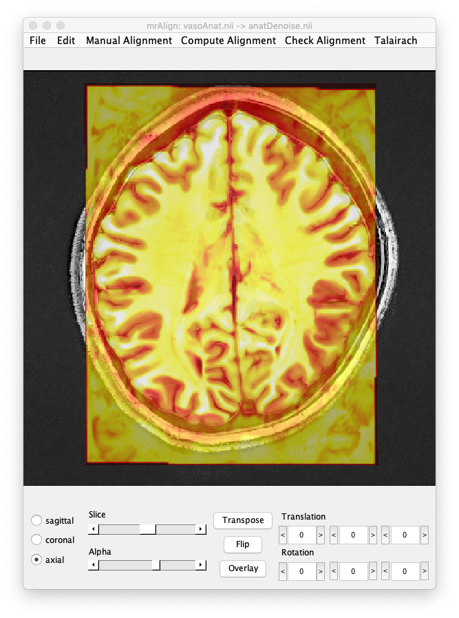
Then align vasoAnat.nii and vasoAnatUpsampled.nii to anatWarped.nii, and export the alignment to the mrTools session.
3. Draw inner and outer layers with fsleyes.app
In this step, we are going to draw inner and outer surfaces on the upsampled vasoAnat using FSLeyes. Note that we'll use the registered and warped MP2RAGE to guide the layer definition since the gray/white definition is better than the vasoAnat. But note that when we flip back and forth, there is not a perfect agreement between the two scans. The layer profiles should respect the vasoAnat as closely as possible, not the MP2RAGE, since the vasoAnat exactly matches the spatial distortions of the functional data. Here is a movie flipping back and forth between the two illustrating the spatial differences:
This step roughly follows the procedures described on Renzo's blog.
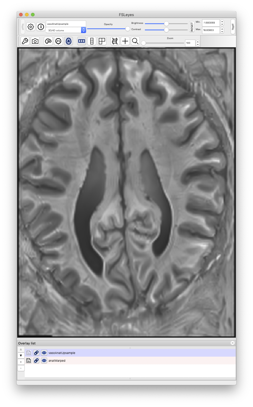
3.1 Load the data into FSLeyes
fsleyes anatWarped.nii vasoAnatUpsample.nii
You can then zoom in on a small FOV containing the chunk of cortex that you are interested in.
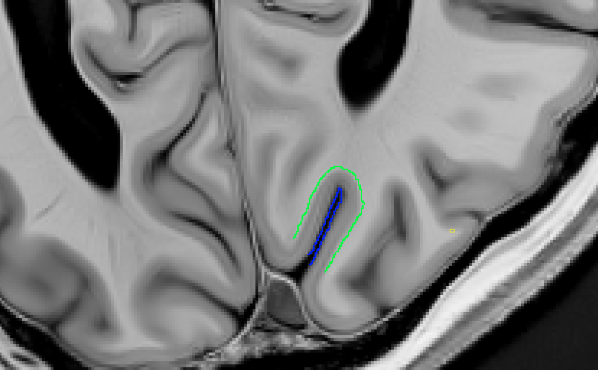
3.2 Draw the inner and outer borders
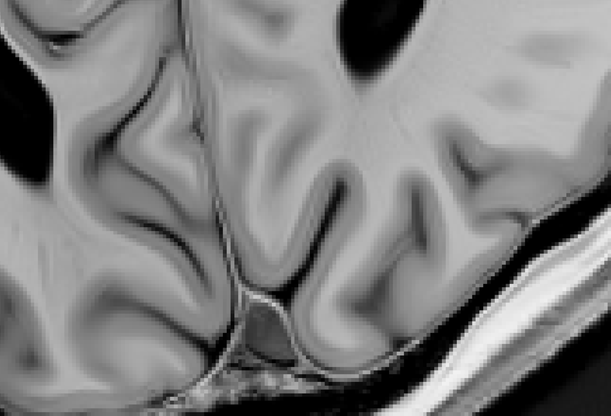
Press opt+e to enter editing mode. Then select vasoAnatUpsample and use the toolbar to create an empty mask with the same resolution. Use the drawing tools to draw inner border with a value of 1 and and outer with value of 2, like this:
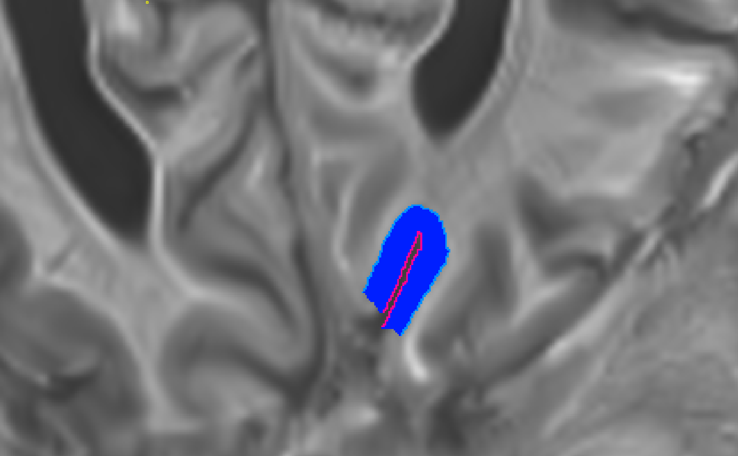
3.3 Make a ribbon intensity mask (RIM)
Join the inner and outer borders with a value of 3, fill the cortical ribbon with a value of 3 with the bucket tool, and save the file:
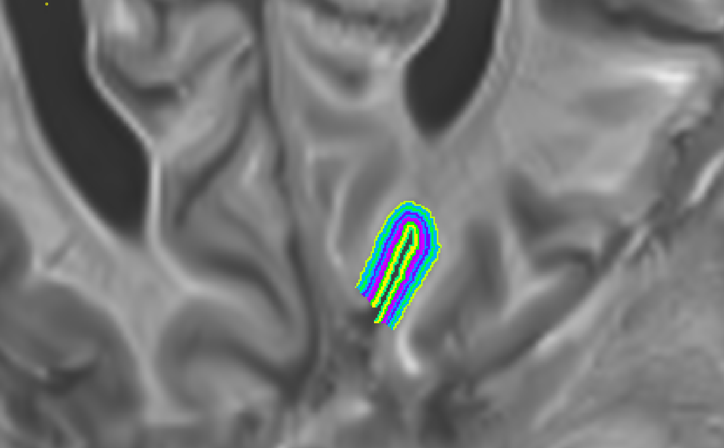
4. Grow layers with LAYNII
5. Create mrTools ROIs from layer mask
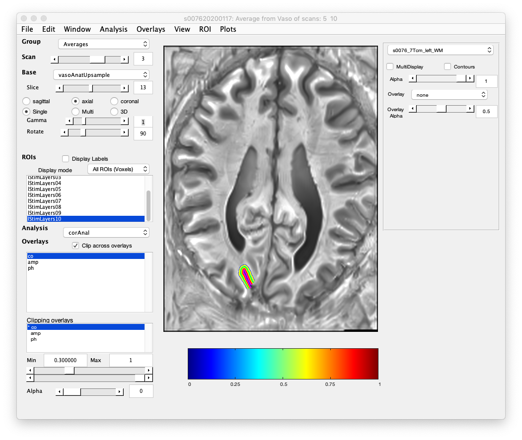
Run the matlab function laynii2ROI to create a set of mrLoadRet ROIs based on the layer mask created by LAYNII.
>> laynii2ROI('Anatomy/sl12-rim_layers.nii');
6. Plot layer profiles
Useful links
This is a tool that may be useful for segmenting images with a small FOV.
