No matter what kind of experiment you do - you always want to look at the data you collect in as raw a format as you can. With neuroimaging this is even more important, because often data are processed with complex multi-step analyses and you can lose track of what features of your data give a result and get into real trouble. Lukily with imaging data, you can just look at your data, cause, well, it's a bunch of images. So let's do that first!

First thing to note is the “Group” drop-down at the top-left. We store data in different “groups” (folders on the harddrive) depending on what stage of analysis the data is in. We want to look at the “Raw” group - so:

Step 1: Select the “Raw” group

In MRI measurements there are different images made with different contrasts (for example, T1 or T2 or T2*-weighted images). For this purpose, just know that a typical anatomical image that you might see is “T1-weighted” where gray matter is gray, white matter is white and cerebral spinal fluid is black. You can take a look at that image by loading it as a “Base Anatomy”. A note here is that we can display summary statistics and data on many different kinds of base anatomies (we will see surfaces and flat-maps in a second). When we do so, we are just doing this for visualization - we transform the statistics on the fly to display on these base anatomies - we always keep the raw data in its original format (thereby avoiding messing with the original data too much by resampling and interpolation only when it is necessary to visualize). We always collect a T1 weighted anatomical image every session - this is used for visualization and for alignment with a canonical anatomy and surfaces (as we will see below).

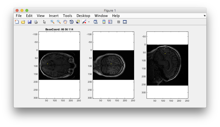
Step 2: Load the T1 anatomy Should already be loaded (i.e. will look like the figure below with pictures of the brain), but if not, go to the menu item: File/Base Anatomy/Load and select the T1 weighted anatomy. Should be called something like “anat01_11954_2_1_T1w_9mm_sag.nii”

You should see the name of the anatomy appear in the Base drop-down and a picture of the brain appear. A few fun things to do here:

Step 3: Examine T1 anatomy Click on the “Multi” radio button. You should see 4 different views of the brain. If you click (make sure that Plots/Interrogate Overlay is unchecked) in any of the views (except the bottom-right one), it will update the other slices to show you that location in the brain. Explore!

Step 4: 3D anatomy view Another view that is sort of fun is to select the 3D radio button and move the 3D slice view around. Not sure that you learn anything different, but it looks kinda cool.

Ok. Cool. So, what about the “functional” data? Well, those are collected at a much faster-rate, typically with a fast imaging sequence known as EPI (Echo Planar Imaging), and have a T2*-weighted contrast. These are sensitive to the paramagnetism of deoxygenated hemoglobin (they get darker where there is more deoxygenated hemoglobin), let's take a look at these.

Step 5: Look at raw EPI images Go to Plots/Display EPI Images. You should see a viewer, where you can look at individual images or slices. Look at individual images. Click displayAllSlices and Animate over frames. This will show you a movie of all the images of the brain.

Note the different image contrast. What color is gray-matter? What color is white matter? How good is the resolution compared to the T1 we just looked at? Do you see evidence of head-motion? Do you see evidence of BOLD contrast (consider that large changes in BOLD are about a couple of % - do you think you could see them)?

It is often helpful to examine our data on renderings of the cortical surface. This is done by processing a high-resolution T1 image of the brain to find the borders between the gray and white matter and the surface of the brain. Then you can segment out just the cortical surface. This is useful since you can throw out data from outside the brain, or within the white matter and visualize on the cortical topography. FreeSurfer is a useful set of tools that can do this automatically on a T1 image (you type one command and then come back in 24 hours or so and it has segmented the brain and made triangulated surfaces. Check here if you wish to know more about surfaces and flat maps. In this section we'll just take a look at the surfaces so you can see a bit about how they are made.

In the Base dropdown, you should be able to select one of the inflated surfaces (e.g. s0371_left_inf or s0371_right_inf). If you do not see those in the dropdown, you may need to load them from the File menu (File/Base Anatomy/Load). To examine how the 3D surface relates to the underlying 3D anatomy, go to Plots/Surface Viewer

Two windows should open, the “View surface” window allows you to set which surfaces you will view data on. There are two visualiation surfaces, outersurface and innerSurface. By having two surfaces, we can provide a slider later which will allow you to smoothly interpolate between the outer and inner surface for visualization. We will therefore use the inflated surface for the outer and the gray matter for the inner surface. The coords surfaces are really important. They determine where the data will come from that you visualize on these surfaces. It is set up so that the gray and white mater surfaces are the coordinate surfaces so that we can interpolate data from within the cortex. The dialog should look like the following:

Examine the segmentation Remember the segmentation should show you the outer and inner surfaces of cortex. Let's examine if the algorithm found it correctly. You should see the 3D anatomy in the other window with white and yellow dots. The white dots indicate the gray matter white matter boundary. The yellow dots indicate the pial surface, or the gray matter/CSF boundary. Scroll through the slices, do you see any errors? I.e. white matter that snuck in, gray matter that was left out, etc? Does the segmentation fail in any specific parts of the brain? How noisy does the gray matter and white matter look?

Often it is convenient to look at data on a flattened piece of cortex (makes it easier to view V1). Let's examine a flat patch. In the Base dropdown menu select s0371_left_occipital.

1. Which way is up Most confusing thing about these patches, is which way is up? To figure this out
   1. Make sure session anatomy is loaded Peak in the Base drop-down and make sure you have the session anatomy anat… If it isn't load it, and switch back to your flat map.
   2. Select searchForVoxel interrogator In the interrogator drop down at bottom left.
   3. Start search Click on any location in the flat patch. A dialog box should come up. Make sure that baseName is set to your session anatomy and that continuousMode is checked.
   4. Find the top of the patch move your mouse (don't click) over the patch, you should see a yellow dot move around in the session anatomy noting the location where that part of the brain comes from.

      
   5. Click red close button Note that if you use ok, you will need to then wait a second - then you will need to set Base back to the flat patch (the searchForVoxel interrogator takes you to the location you clicked in the other anatomy.
   6. Rotate to top Now use the rotate slider at the left to rotate the patch until the location that you determined was at the top of the brain is at the top of the viewer.

Ok. Now we're ready to look at the pRF analysis.

1. Concatenation and Averages Typically we average together a few scans where we showed the exact same set of bars to improve our SNR. This should already be done. In fact, we have concatenated a set of different runs, so just switch to the Concatenation group in the Group dropdown menu.
2. pRF analysis The pRF analysis takes some time to run, so it should already be run for you. (If not, you would run it from the Analysis/pRF analysis menu).
3. Examine r2 First thing to do is to see how much of the variance is accounted for. In the Overlays box at left, click on r2 to view the r2 overlay.

   

   Note that this example is from our regular pRF scans in which we run 8 runs and average which will give better SNR then the 4 runs that you ran.
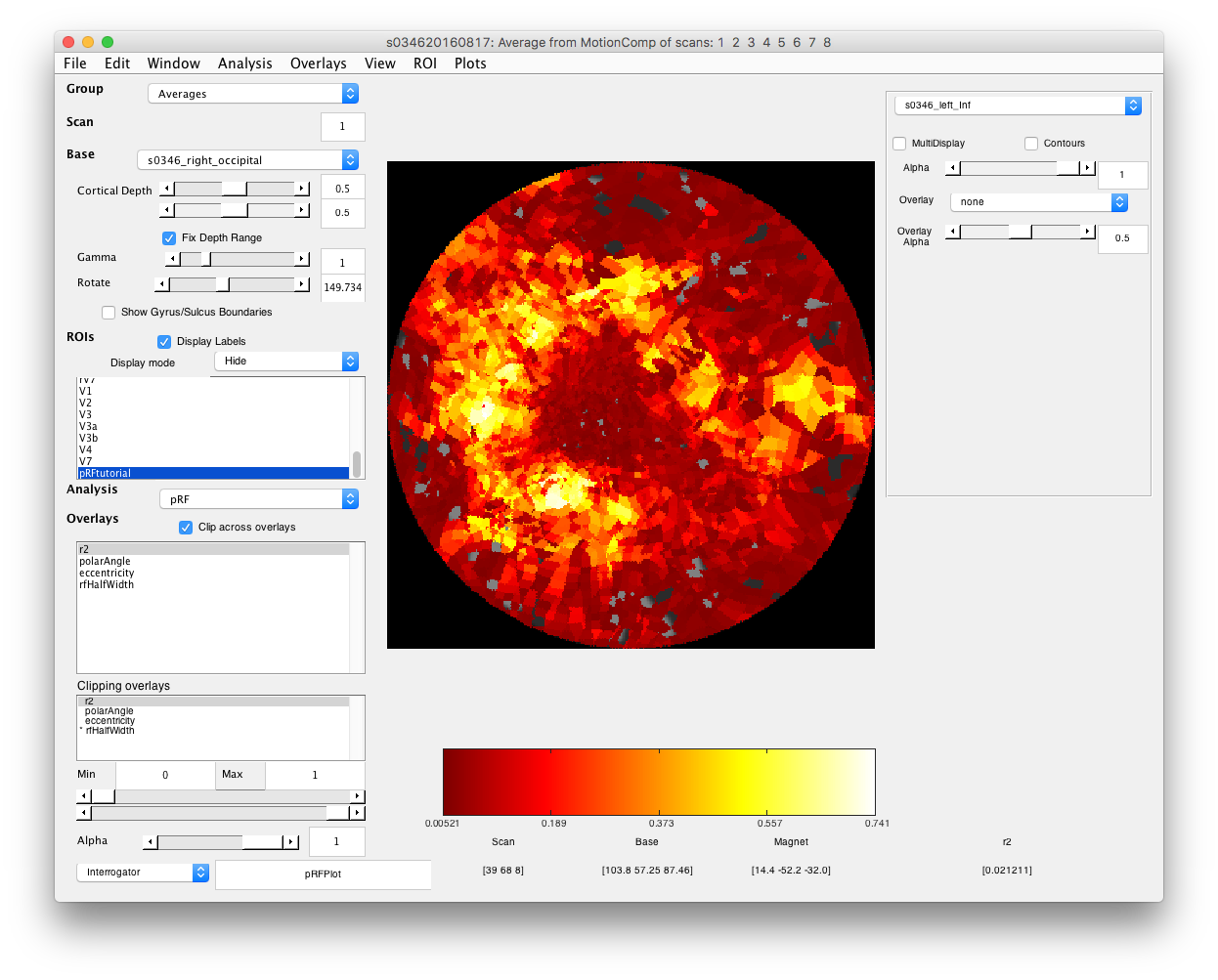
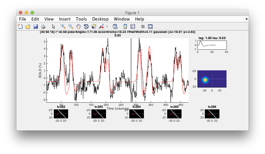
4. Examine good voxel fits Making sure that the Interrogator is set to “pRFPlot” click on points in the flat map with high r2 (whitish). Does the fit (red) match the data (black)? If you move your mouse over the time series you should be able to see the stimulus and the receptive field at bottom that generated the model predictions. Makes sense?

   
5. Examine poor voxel fits Click on a few voxels with low r2. What happened there? Why are the fits bad? Do they have visual responses?
6. Select r2 cutoff voxels with poor r2 are just basically noise, so you may want to not view them in the overlays if it is easier. Set the Min slider at bottom left, making sure that “Clipping Overlays” is set to r2 to a value that gets rid of voxels with poor r2 (this can be pretty arbitrary for this purpose - if you really wanted to you could base clipping on some statistical test of goodness-of-fit.
7. Examine eccentricity Chose “eccentricity” from the Overlays and examine that. Click on voxels to see if they match what is being displayed.
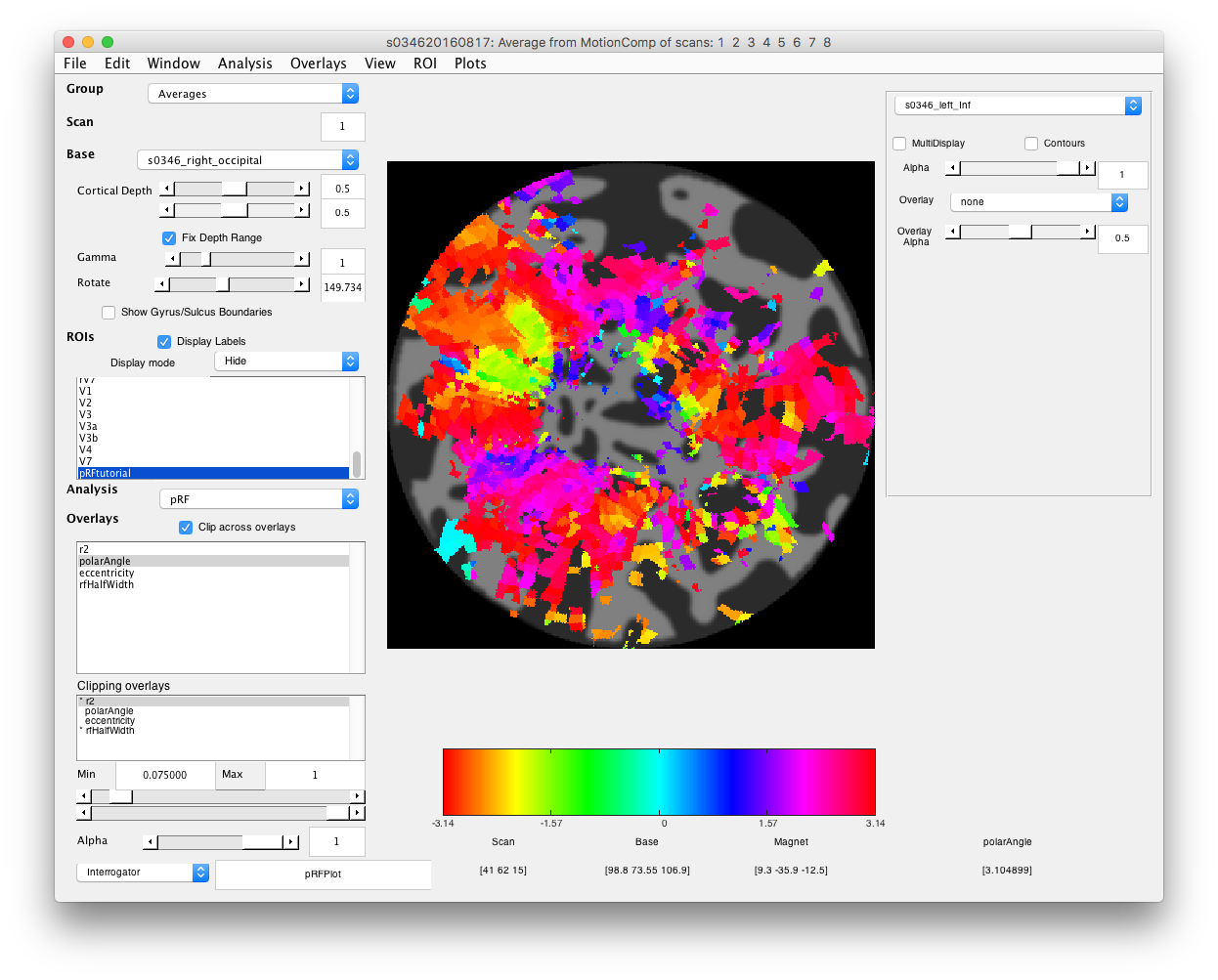
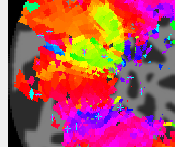
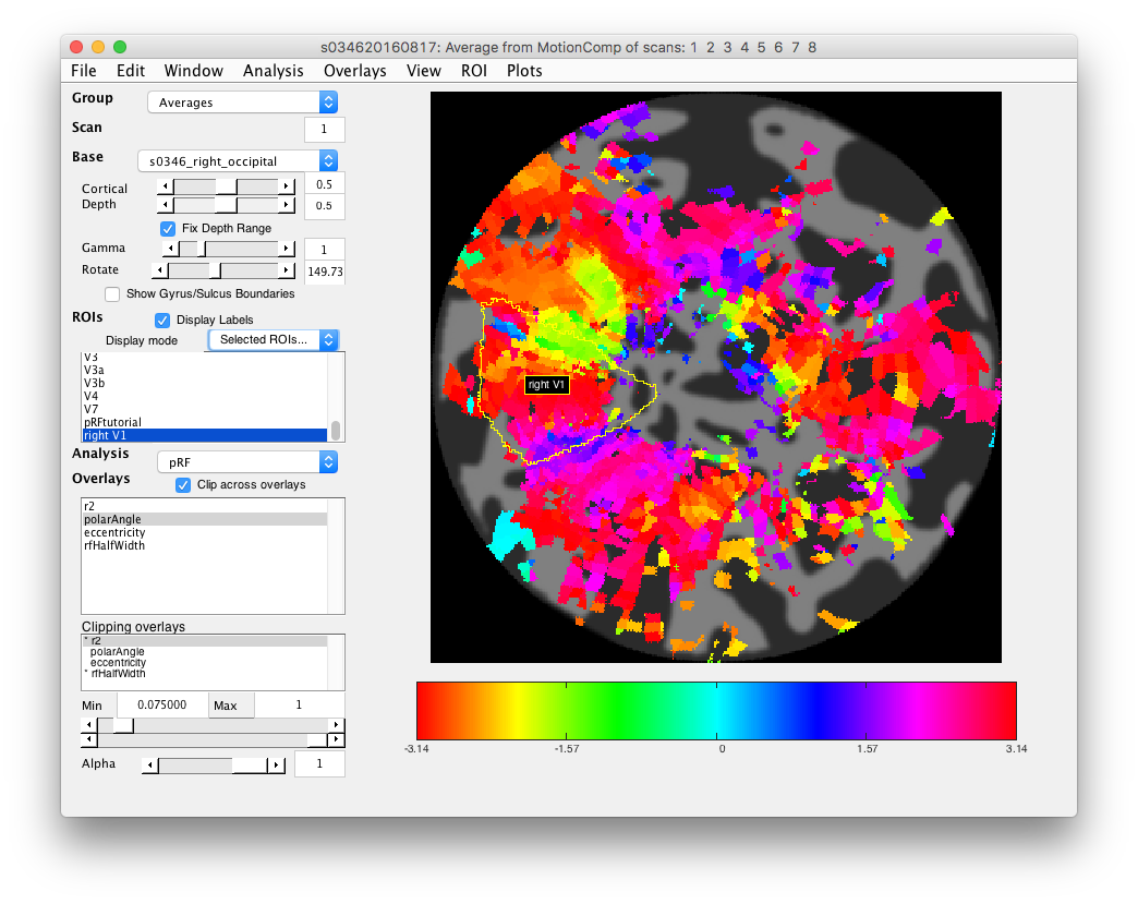
8. Examine polar angle Choose “polarAngle” from the Overlays and examine that. This is how we are going to determine where V1 is. Remember that V1 is a full hemifield which is flipped on the cortex (goes from upper to lower visual meridian as you go from the bottom to the top of the calcarine sulcus). When you get to V2, the direction reverses and this is how you know where V1 is. In practice, you are going to look for colored stripes in the data where the vertical meridians are and draw an ROI around there for V1. You should look for two of the same color lower visual meridians (V1/V2 and V2/V3 borders, green in example below) in the top and two of the same color upper visual meridians in the bottom (magenta in the example below).

   

   Click a few voxels on these meridians to determine if the visual RFs are where you think they should be. Note that things may not look as pretty as in the above example, just because we collected less data. Ask if you can't figure out where V1 is!
9. Draw V1 region of interest Turn off Plot/Interrogate Overlay. Go to ROI/Create/Polygon set the name to left/right V1 and click OK. Then on the flat map, draw your ROI by clicking. DOuble-click to finish the ROI.

   

   Make sure that Selected ROIs (Perimeter) is selected in the drop down at left for Display Mode and you should see your V1 ROI

   
10. Draw V1 in other hemisphere Do the same for V1 in the other hemisphere.