Table of Contents
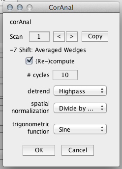
5. Correlation Analysis
8. Show correlation analysis on surfaces
Now load one of your surface with superimposed correlation analysis and toggle the Overlay from ph to co, then slide the Overlay min to 0.4 for visualizing (though remember to undo that later).
Darker red indicates a correlation close to 1–that is, a region whose activity responds in correlation with the stimulus. That is good. We want dark red areas because those are what interest us.
To see how good that correlation is, go to Plots/Interrogate Overlay and use the crosshairs to click on a dark red region. You will get a window like the following.
Note that here, the black data points at the top closely resemble the estimated red sine wave. In the bottom right, the contrast-to-noise ratio (CNR) is near 100, which is great. You can see how this is not the case when you use the Interrogate Overlay tool to click an area with little or no correlation.
When you close out, put the co Overlay min back to 0 if you haven't done so already.
If you do not have Freesurfer set up, visualization will be different since your data will be on a two-dimensional map of the cortical surface. Regardless, in the image you see you will find that darker red indicates a correlation close to 1–that is, a region whose activity responds in correlation with the stimulus. That is good. We want dark red areas because those are what interest us.
To see how good that correlation is, go to Plots/Interrogate Overlay and use the crosshairs to click on a dark red region. You will get a window like the following.
Note that here, the black data points at the top closely resemble the estimated red sine wave. In the bottom right, the contrast-to-noise ratio (CNR) is near 100, which is great. You can see how this is not the case when you use the Interrogate Overlay tool to click an area with little or no correlation.
When you close out, put the co Overlay min back to 0 if you haven't done so already.
7. Show correlation analysis on a flat map
To make a flat map of the three-dimensional brain image, go to Plots/Interrogate Overlay and select makeFlat from the bottom-left menu.
Now, simply use the crosshairs and click on an area that you want to flatten.
This will appear.
Here, you can change all sorts of parameters like the patch color and size. Set the radius size to about 90. When you are done, click OK and proceed to the following dialog.
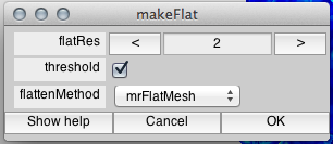
The flatRes, or “resolution”, of the flat patch, is usually set to 2. You can turn it up if the flat patch you receive looks choppy and pixellated.
With the Overlay set to ph, now toggle between your Scans (wedges, rings, etc.) to see how your flat map signals vary between them. You will be drawing ROIs based on their signals in just a bit.
Before you move on, if you have finalized your surfaces and flat maps, be sure to go through File/Base Anatomies/Save for each individual base to save it in your directory. Additionally, you can use File/Anat DB/Add Base Anatomies to Anat DB to upload them.


