The ready to use protocol is here: gruretinotopystanford.xls

This detailed checklist for the retinotopy in Stanford need to be re-written here.

fmrichecklist07.ods

At this point you should have already completed segmentation, dofmricni, and mrAlign. See the specific tutorials for those tasks.

When you are satisfied with the fit, proceed and run

mrInit

to initialize the session for mrTools. On the menu that appears, fill in the description, subject, operator, etc.

In the following window for group parameters, fill out information group parameters for the frames as needed. If you cannot find a description of each scan, refer to an information sheet which should be in the folder [username]/data/retinotopy/[session id]/Docs. Here, you should be able to find which scans are clockwise-wedges, for example, or contracting rings. Fill this information in; it will be helpful later. Then select OK to finish the initialization. Note that for this set it is not necessary to specify any junkFrames to remove, as the current scanning program already removes them.

Once that has been finished, run

mrLoadRet

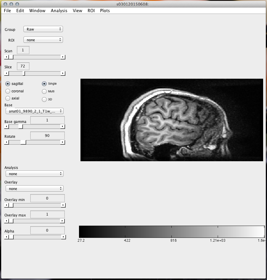
and see the following window appear.

On this screen, explore the different types of views and different slices of each to see the brain images. Slices from the middle of the coronal view often give a good view.

Next, pull up a menu that lets you check and animate all of the scans. Here, you can check to see which scans, if any, are problematic and should be ignored in the final analysis. (FIND OUT FROM JUSTIN WHAT MENU THIS WAS?)

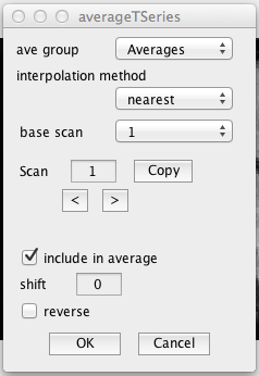
Go to Analysis/Average Time Series and look at the following menu.

Through this program we will be averaging the data for scans that involved the same types of stimuli. We will also be using this opportunity to adjust volumes so that we can compensate for hemodynamic lag. Make multiple sets of averages, all with differing levels of adjustment, so you can find which shift value works best (usually between -3 and -6). Be sure to reverse counterclockwise and contracting patterns (as is the convention).

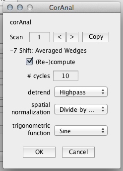
Once your averaged groups are created (switch the group from MotionComp to Averages to see), we can run them through correlation analysis so that we can evaluate how well the data fit.

Go to Analysis/Correlation Analysis and fill out the information as follows for all the scans.

Now load one of your surface with superimposed correlation analysis and toggle the Overlay from ph to co, then slide the Overlay min to 0.4 for visualizing (though remember to undo that later).

Darker red indicates a correlation close to 1–that is, a region whose activity responds in correlation with the stimulus. That is good. We want dark red areas because those are what interest us.

To see how good that correlation is, go to Plots/Interrogate Overlay and use the crosshairs to click on a dark red region. You will get a window like the following.

Note that here, the black data points at the top closely resemble the estimated red sine wave. In the bottom right, the contrast-to-noise ratio (CNR) is near 100, which is great. You can see how this is not the case when you use the Interrogate Overlay tool to click an area with little or no correlation.

When you close out, put the co Overlay min back to 0 if you haven't done so already.

If you do not have Freesurfer set up, visualization will be different since your data will be on a two-dimensional map of the cortical surface. Regardless, in the image you see you will find that darker red indicates a correlation close to 1–that is, a region whose activity responds in correlation with the stimulus. That is good. We want dark red areas because those are what interest us.

To see how good that correlation is, go to Plots/Interrogate Overlay and use the crosshairs to click on a dark red region. You will get a window like the following.

Note that here, the black data points at the top closely resemble the estimated red sine wave. In the bottom right, the contrast-to-noise ratio (CNR) is near 100, which is great. You can see how this is not the case when you use the Interrogate Overlay tool to click an area with little or no correlation.

When you close out, put the co Overlay min back to 0 if you haven't done so already.

To make a flat map of the three-dimensional brain image, go to Plots/Interrogate Overlay and select makeFlat from the bottom-left menu.

Now, simply use the crosshairs and click on an area that you want to flatten.

This will appear.

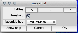
Here, you can change all sorts of parameters like the patch color and size. Set the radius size to about 90. When you are done, click OK and proceed to the following dialog.

The flatRes, or “resolution”, of the flat patch, is usually set to 2. You can turn it up if the flat patch you receive looks choppy and pixellated.

With the Overlay set to ph, now toggle between your Scans (wedges, rings, etc.) to see how your flat map signals vary between them. You will be drawing ROIs based on their signals in just a bit.

Before you move on, if you have finalized your surfaces and flat maps, be sure to go through File/Base Anatomies/Save for each individual base to save it in your directory. Additionally, you can use File/Anat DB/Add Base Anatomies to Anat DB to upload them.

For this next stage, we will be using correlation analyses and phase overlays to determine visual fields on the cortical surface based on their patterns of activity. This sounds good and we have used it extensively in the past, but do take not that the population receptive fields (pRFs) we run later will be much better at visualizing activity. That said, let's proceed.

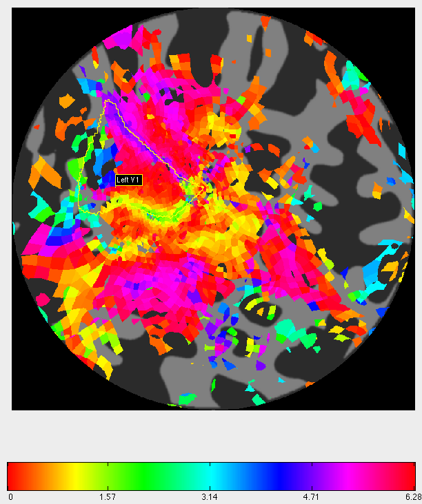
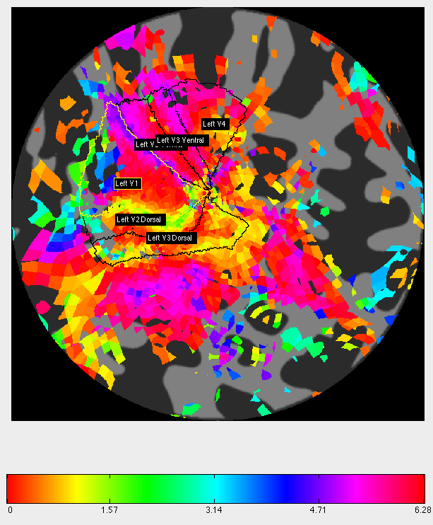
First, accustom yourself with the flat map and its key locations. If you go to the rings scan, you will see a gradient originating from a center point, the fovea. This is important, because it is where the visual field ROIs originate as well. Go to the wedges scan to see that there are what look like colored spokes leading in towards the center. Turn the Overlay to co and set the Overlay min to about 0.2 to clean up some of the scan.

Go to ROI/Create/Polygon to start drawing ROIs. To draw, simply click points along the outline of your ROI, then double-click to finalize. For these steps it is probably best to refer to a sample image created by a professional (FIND PICTURE FROM JUSTIN).

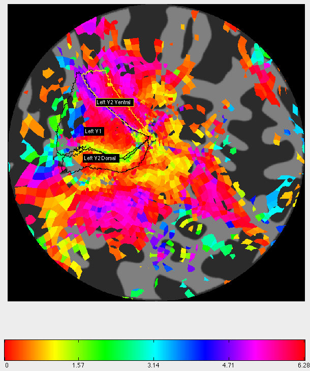
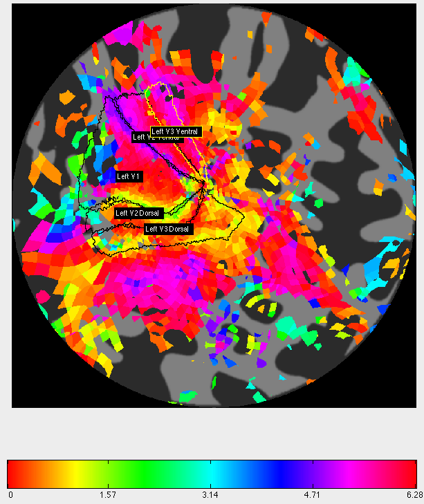
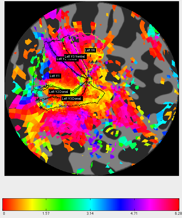
Tips: use the wedges scan and the colors to find out the polar angles of the ROIs, but use the rings scan to find the eccentricity (distance) of each. Recall that V1 and V4 comprise full hemifields (debate on the latter) and that V2 and V3 comprise half hemifields.

V1: this ROI comprises a full hemifield, from 1/2 pi to 3/2 pi (thus, colors corresponding to 1.57 and 4.71 on the bottom scale). On the wedges scan, you will see a region bounded by these two colors–green and blue in this example. If you have trouble finding it, you can look for area MT, which should be a patch of color directly opposite from it.

V2 (Ventral and Dorsal): half-hemifields on each side of V1. Note that which side is ventral and which side is dorsal will be reversed if you are working with a right occipital lobe.

V3 (Ventral and Dorsal): more half-hemifields extending even more outwards.

V4: full hemifield on the ventral surface.

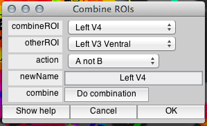
By this point you most likely have some overlap between your ROIs. Let's take care of that. Go to ROI/Combine and look at the following interface.

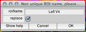
By filling out the information as follows and clicking Do combination, then checking Replace and OK, we will be sending voxels that overlap between Left V3 Ventral and Left V4 into Left V4. That way, we can eliminate any overlap between the two.

We repeat the process for all of the overlaps between the ROIs. It is useful to go from one end to the other systematically.

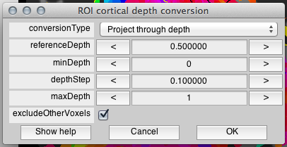
Now we can extend our ROIs through the gray matter so that they are not drawn on just one layer. Set your Cortical Depth slider at 0.5 and go to ROI/Convert/Convert cortical depth. The information should be entered as follows.

Select OK and check all the ROIs that you want to convert. Afterwards, you should be able to move the Cortical Depth slider up and down and see how your ROIs are featured in different levels within the gray matter.

When you are satisfied, go to File/ROI/Save all to save your work.

To update your local repository

localRepo = mlrAnatDBgetRepo('025')

Now go look in ~/data/mlrAnatDB/s0025/localizers

All session files are saved there.

Use mlrAnatDBPut to add ROIS or mlrBaseAnatomies to mercurial database or use the GUI file/AnatDB/Add ROIs to add Rois or /file/ANatDB/Add mlrBaseAnatomies to add surfaces and flat maps

ROIS should contain:

- ROIS

- Localizers

Localizer folder should contain :

- The most recently updated session analysis.

mlrBaseAnatomies should contain:

- Surfaces (.off .vff files)

- Flat maps

To do the Alignment on the canonical download the canonical from the database

[localRepo localRepoLargeFiles] = mlrAnatDBgetRepo('301')

then

mrALign

follow the instruction from the retinotopy tutorial to Align the inplane (from local session anatomy folder) to the canonical (~/data/mlrAnataDB/s0301/s0301.nii)

Everytime we load mrloadRet it seems we have to load mlrPlugin('altPlugins')…Isn't there a way to make that systematic ?

Flat maps (90 degrees radius)

- parietal

- occipital

- ventral