Table of Contents
Setup
At this point you should have already completed segmentation, dofmricni, and mrAlign. See the specific tutorials for those tasks. Set your Plugins (just tick them all) and call mrLoadRet
mlrPlugin('altPlugins=1')
mrLoadRet
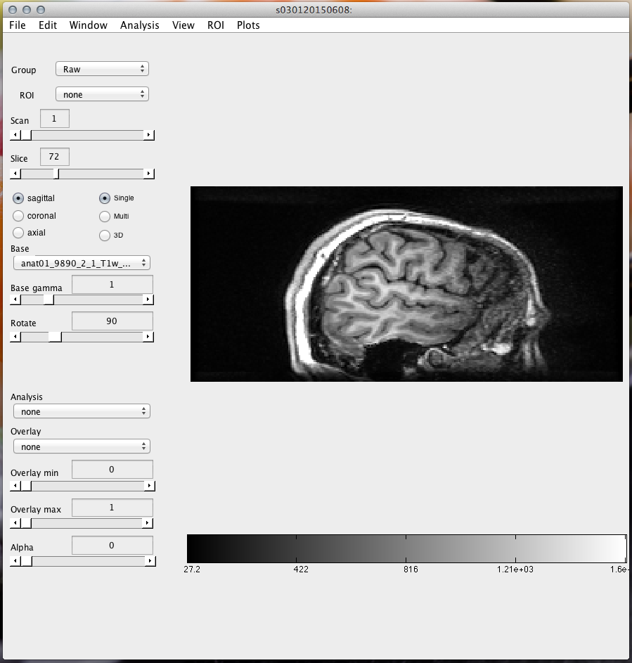
and see the following window appear.
On this screen, explore the different types of views and different slices of each to see the brain images. Slices from the middle of the coronal view often give a good view.
Check Your Data
Go to Plots > Display EPI Scans. Use the “animate” button to go through your scans individually and make sure that (1) the motion compensation worked and (2) there aren't any bizarre artifacts.
Average Time Series
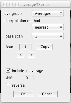
Go to Analysis/Average Time Series and look at the following menu.
Through this program we will be averaging the data for scans that involved the same types of stimuli. We will also be using this opportunity to adjust volumes so that we can compensate for hemodynamic lag. Make multiple sets of averages, all with differing levels of adjustment, so you can find which shift value works best (usually between -3 and -6). Be sure to reverse counterclockwise and contracting patterns (as is the convention).
Once your averaged groups are created (switch the group from MotionComp to Averages to see), we can run them through correlation analysis so that we can evaluate how well the data fit.
Correlation Analysis
Correlation analysis is the 'simple' straightforward way of doing retinotopy, but it is also not as good as the pRF Fit. I have separated the correlation instructions out into this tutorial but honestly, just do the pRF.
But–if you need to use correlation for other localizers (Motion localizer, Somatosensory localizer), you'll still need to do those steps. See the tutorial above!
Population Receptive Field (PRF) Analysis
See also |mrTools pRF Tutorial
Average Runs
If you have any duplicate runs (two CCW CW, or four Bar runs for example), go ahead and average them into a new Averages group. Copy your other scans into that group as well (Edit > Scan > Copy Scans, then Edit > Scan > Paste Scans into your Averages Group).
Concatenate Runs
Analysis > Concatenate. The defaults are fine, make sure to create a new group and to give your scan an appropriate name “Concat for Retinotopy”. If you have non-retinotopy localizers make sure you do not include them in your concatenation (e.g. motion localizers).
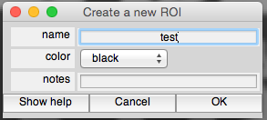
Create a test ROI
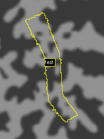
Before you run a PRF that takes hours to complete lets make sure that things are working as expected. Draw a test ROI roughly where you think V1 might be.
Run the test pRF
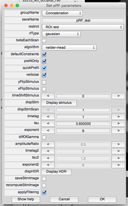
Give your analysis a name like pRF_test, and make sure that you set both prefitOnly and quickPrefit. These will ensure that the test runs very quickly. Set restrict to your ROI: test. The other parameters can be left at their defaults.
If you have the parallel computing toolbox installed you can speed things up significantly using matlabpool. If you don't, tough luck! This initial test will still only take a few minutes to run.
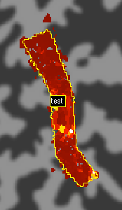
You should get this:
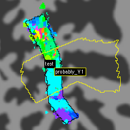
Note that the R^2 map is not particularly helpful on the prefit. For some reason it ends up having very low (but relative to itself not meaningless) values. Anyways, it looks like we aimed correctly and that was V1, so let's do a full pRF. Draw a new ROI that covers your entire flat map and run the pRF using “prefit only” but not the quick prefit.
Run a full pRF
If you want you can run a pRF prefit for the entire surface, this usually only takes a few hours. Make sure to run a separate pRF_left and pRF_right for each hemisphere. The full pRF will never finish if it isn't restricted to an ROI. I recommend drawing the ROI by hand on each flat map, you can always expand the ROI and re-run the pRF later if you need to. We recommend extending ROIs through at least part of the cortical depth (.2→.8) prior to running the pRF analysis. Once the pRF finishes you can start drawing ROIs. If you have time, make sure your pRF ROI covers everything you want and then run the full pRF with prefit only turned off.
8. Draw ROIs
For this next stage, we will be using correlation analyses and phase overlays to determine visual fields on the cortical surface based on their patterns of activity. This sounds good and we have used it extensively in the past, but do take not that the population receptive fields (pRFs) we run later will be much better at visualizing activity. That said, let's proceed.
First, accustom yourself with the flat map and its key locations. If you go to the rings scan, you will see a gradient originating from a center point, the fovea. This is important, because it is where the visual field ROIs originate as well. Go to the wedges scan to see that there are what look like colored spokes leading in towards the center. Turn the Overlay to co and set the Overlay min to about 0.2 to clean up some of the scan.
Go to ROI/Create/Polygon to start drawing ROIs. To draw, simply click points along the outline of your ROI, then double-click to finalize. For these steps it is probably best to refer to a sample image created by a professional (FIND PICTURE FROM JUSTIN).
Tips: use the wedges scan and the colors to find out the polar angles of the ROIs, but use the rings scan to find the eccentricity (distance) of each. Recall that V1 and V4 comprise full hemifields (debate on the latter) and that V2 and V3 comprise half hemifields.
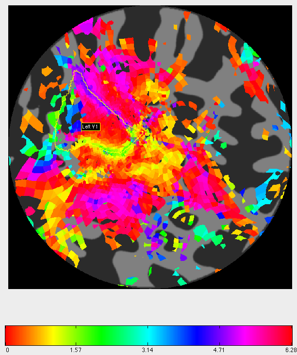
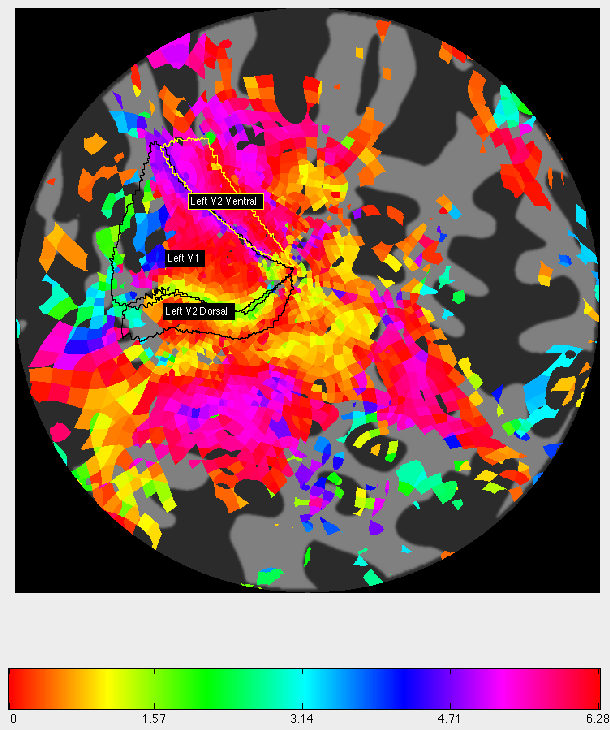
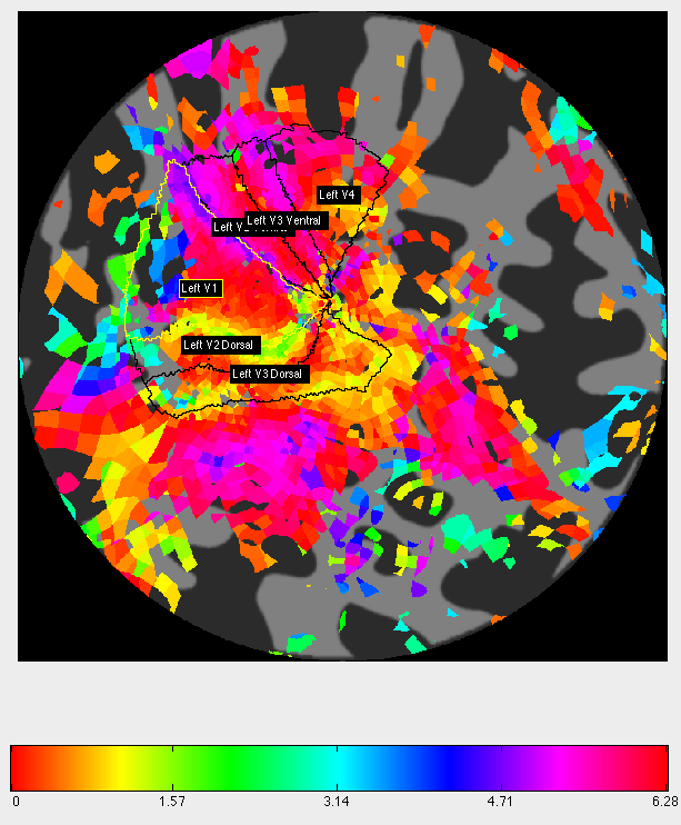
V1: this ROI comprises a full hemifield, from 1/2 pi to 3/2 pi (thus, colors corresponding to 1.57 and 4.71 on the bottom scale). On the wedges scan, you will see a region bounded by these two colors–green and blue in this example. If you have trouble finding it, you can look for area MT, which should be a patch of color directly opposite from it.
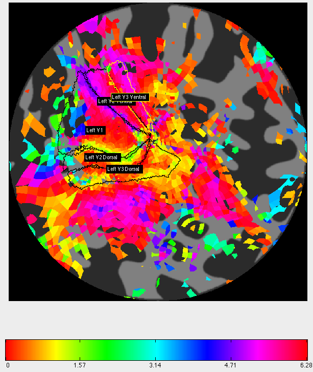
V2 (Ventral and Dorsal): half-hemifields on each side of V1. Note that which side is ventral and which side is dorsal will be reversed if you are working with a right occipital lobe.
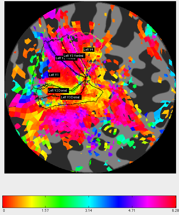
V3 (Ventral and Dorsal): more half-hemifields extending even more outwards.
V4: full hemifield on the ventral surface.
9. Clean Up ROIs
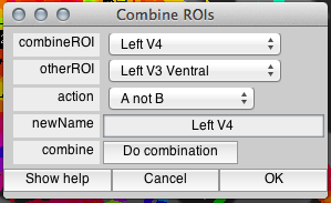
By this point you most likely have some overlap between your ROIs. Let's take care of that. Go to ROI/Combine and look at the following interface.
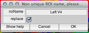
By filling out the information as follows and clicking Do combination, then checking Replace and OK, we will be sending voxels that overlap between Left V3 Ventral and Left V4 into Left V4. That way, we can eliminate any overlap between the two.
We repeat the process for all of the overlaps between the ROIs. It is useful to go from one end to the other systematically.
10. Extend ROIs
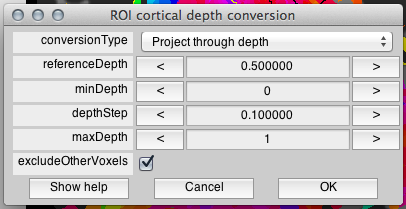
Now we can extend our ROIs through the gray matter so that they are not drawn on just one layer. Set your Cortical Depth slider at 0.5 and go to ROI/Convert/Convert cortical depth. The information should be entered as follows.
Select OK and check all the ROIs that you want to convert. Afterwards, you should be able to move the Cortical Depth slider up and down and see how your ROIs are featured in different levels within the gray matter.
When you are satisfied, go to File/ROI/Save all to save your work.
Add to AnatDB
If you followed the tutorials so far, you should have already added your session to AnatDB. If so you can just go File > AnatDB > Add ROIs to AnatDB and you're good to go! If not you will need to add the session first. You can check if your push to the AnatDB was successful here: Anat DB
pRF Average vs. Concatenation Comparison
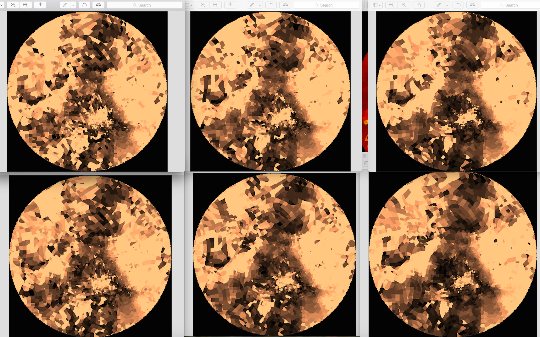
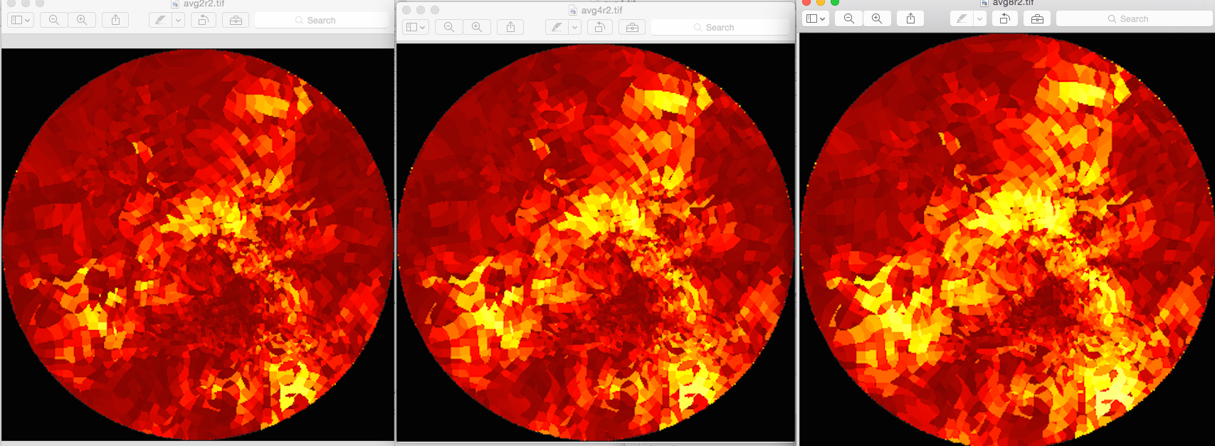
Dan used a single subject and compared 8 v 4 v 2 bar runs in averaged and concatenated format. The analysis suggests that our standard retinotopy should include a minimum of 4 bar runs, and that a small improvement can be made by collecting 6+. Analysis should be done by averaging for a HUGE reduction in pRF run time (also it takes less memory).
R^2 map for Averages, 2, 4, 8:
Polar Angle map for Averages (top), Concat (bot), 2, 4, 8:
